This HTML version of is provided for convenience, but it is not the best format for the book. In particular, some of the symbols are not rendered correctly.

You might prefer to read the PDF version.

Chapter 10  Approximate Bayesian Computation

10.1  The Variability Hypothesis

I have a soft spot for crank science. Recently I visited Norumbega Tower, which is an enduring monument to the crackpot theories of Eben Norton Horsford, inventor of double-acting baking powder and fake history. But that’s not what this chapter is about.

This article is about the Variability Hypothesis, which

"originated in the early nineteenth century with Johann Meckel, who argued that males have a greater range of ability than females, especially in intelligence. In other words, he believed that most geniuses and most mentally retarded people are men. Because he considered males to be the ’superior animal,’ Meckel concluded that females’ lack of variation was a sign of inferiority."

From http://en.wikipedia.org/wiki/Variability_hypothesis.

I particularly like that last part, because I suspect that if it turns out that women are actually more variable, Meckel would take that as a sign of inferiority, too. Anyway, you will not be surprised to hear that evidence for the Variability Hypothesis is not strong.

Nevertheless, it came up in my class recently when we looked at data from the CDC’s Behavioral Risk Factor Surveillance System (BRFSS), specifically the self-reported heights of adult American men and women. The dataset includes responses from 154407 men and 254722 women. Here’s what we found:

• The average height for men is 178 cm; the average height for women is 163 cm. So men are taller, on average. No surprises so far.
• For men the standard deviation is 7.7 cm; for women is it 7.3 cm. So in absolute terms, men’s heights are more variable.
• But to compare variability between groups, it is more meaningful to use the coefficient of variation (CV), which is the standard deviation divided by the mean. It is a dimensionless measure of variability relative to scale. For men CV is 0.0433; for women it is 0.0444.

That’s very close, so we could conclude that this dataset provides little support for the Variability Hypothesis. But we can use Bayesian methods to make that conclusion more precise. And answering this question gives me a chance to demonstrate some techniques for working with large datasets.

I will proceed in a few steps:

1. We’ll start with the simplest implementation, but it only works for datasets smaller than 1000 values.
2. By computing probabilities under a log transform, we can scale up to the full size of the dataset, but the computation gets slow.
3. Finally, we speed things up substantially with Approximate Bayesian Computation, also known as ABC.

You can download the code in this chapter from http://thinkbayes.com/variability.py.

10.2  Mean and standard deviation

In Chapter 9 we estimated two parameters simultaneously using a joint distribution. In this chapter we use the same method to estimate the parameters of a normal distribution: the mean, mu, and the standard deviation, sigma.

For this problem, I defined a Suite called Height that represents a map from each mu, sigma pair to its probability:

class Height(thinkbayes.Suite, thinkbayes.Joint):

    def __init__(self, mus, sigmas):
        thinkbayes.Suite.__init__(self)

        self.mus = mus
        self.sigmas = sigmas

        pairs = [(mu, sigma) 
                 for mu in mus
                 for sigma in sigmas]

        thinkbayes.Suite.__init__(self, pairs)

mus is a sequence of possible values for mu; sigmas is a sequence of values for sigma. The prior distribution is uniform over all mu, sigma pairs.

The likelihood function is easy. Given hypothetical values of mu and sigma, we compute the likelihood of a particular value, x. That’s what EvalGaussianPdf does, so all we have to do is use it:

# class Height

    def Likelihood(self, hypo, data):
        x = data
        mu, sigma = hypo

        like = thinkbayes.EvalGaussianPdf(mu, sigma, x)
        return like

If you have studied statistics from a mathematical perspective, you know that when you evaluate a PDF, you get a probability density. In order to get a probability, you have to integrate probability densities over some range.

But for our purposes, we don’t need a probability; we just need something proportional to the probability we want. A probability density does that job nicely.

The hardest part of this problem turns out to be choosing appropriate ranges for mus and sigmas. If the range is too small, we omit some possibilities with non-negligible probability and get the wrong answer. If the range is too big, we get the right answer, but waste computational power.

So this is an opportunity to use classical estimation techniques to make Bayesian techniques more efficient. Specifically, we can use classical estimators to find a likely location for mu and sigma, and use the standard errors of those estimates to choose a likely spread.

If the true parameters of the distribution are µ and σ, and we take a sample of n values, an estimator of µ is

and an estimator of σ² is

The standard error of the estimated µ is

and the standard error of the estimated σ is

Here’s the code to compute all that:

def FindPriorRanges(xs, num_points, num_stderrs=3.0):

    # compute xbar and S
    n = len(xs)
    xbar, S2 = thinkstats.MeanVar(xs)
    S = math.sqrt(S2)

    # compute ranges for xbar and S
    stderr_xbar = S / math.sqrt(n)
    mus = MakeRange(xbar, stderr_xbar)

    stderr_S = S / math.sqrt(2 * (n-1))
    sigmas = MakeRange(S, stderr_S)

    return mus, sigmas

xs is the dataset. num_points is the desired number of values in the range. num_stderrs is the width of the range on each side of the estimate, in number of standard errors. The return value is a pair of sequences, mus and sigmas.

Here’s MakeRange:

    def MakeRange(estimate, stderr):
        spread = stderr * num_stderrs
        array = numpy.linspace(estimate-spread,
                               estimate+spread,
                               num_points)
        return array

Again, we’re using numpy.linspace to make an array with num_points elements equally spaced between estimate-spread and estimate+spread, including both.

10.3  Update

Finally here’s the code to make and update the suite:

    mus, sigmas = FindPriorRanges(xs, num_points)
    suite = Height(mus, sigmas)
    suite.UpdateSet(xs)
    print suite.MaximumLikelihood()    

This process might seem bogus, because we use the data to choose the range of the prior distribution, and then use the data again to do the update. In general, using the same data twice is, in fact, bogus.

But in this case it is ok. Really. We use the data to choose the range for the prior, but only to avoid computing a lot of probabilities that would have been very small anyway. I chose a value for num_stderrs big enough to cover all values with non-negligible likelihood. After that, making it bigger has no effect on the results.

In effect, we are approximating a prior that is uniform over all values of mu and sigma, but for computational efficiency we ignore all the values that don’t matter.

10.4  The posterior distribution of CV

Once we have the posterior joint distribution of mu and sigma, we can compute the distribution of CV for men and women, and then the probability that one exceeds the other.

To compute the distribution of CV, we enumerate pairs of mu and sigma:

def ComputeCoefVariation(suite):
    pmf = thinkbayes.Pmf()
    for (mu, sigma), p in suite.Items():
        pmf.Incr(sigma/mu, p)
    return pmf

Then we can use thinkbayes.PmfProbGreater to compute the probability that men are more variable.

But there are a few problems we have to solve first:

1. As the size of the dataset increases, we run into a series of computational problems due to the limitations of floating-point arithmetic.
2. The dataset contains a number of extreme values that are almost certainly errors. We will need to make the estimation process robust in the presence of these outliers.
3. When we collapse the distributions to a single probability, we lose information about uncertainty. For example, if we report “The probability that men are more variable is 96%,” that report would not take into account the likelihood of the Variability Hypothesis before we saw the data.

We’ll deal with the first two problems in this chapter and come back to the third in the next chapter, which is about Bayesian hypothesis testing.

10.5  Big data, small likelihood

If we select the first 100 values from the BRFSS dataset and run the analysis I just described, it runs without errors and we get posterior distributions that look reasonable.

If we select the first 1000 values and run the program again, we get an error in Pmf.Normalize:

ValueError: total probability is zero.

The problem is that we are using probability densities to compute likelihoods, and densities from continuous distributions tend to be small. And if you take 1000 small values and multiply them together, the result is very small. In this case it is so small it can’t be represented by a floating-point number, so it gets rounded down to zero, which is called “underflow.” And if all probabilities in the distribution are 0, it’s not a distribution any more.

A possible solution is to renormalize the Pmf after each update, or after each batch of 100. That would work, but it would be slow.

A better alternative is to compute likelihoods under a log transform. That way, instead of multiplying small values, we can add up log likelihoods. Pmf provides methods Log, LogUpdateSet and Exp to make this process easy.

Here’s what the update looks like:

    suite.Log()
    suite.LogUpdateSet(xs)
    suite.Exp()
    suite.Normalize()

It’s important not to call Pmf.Normalize while the Pmf is under the log transform; the result would be nonsensical.

Here’s the implementation of Log:

# class Pmf

    def Log(self):
        m = self.MaxLike()
        for x, p in self.d.iteritems():
            if p:
                self.Set(x, math.log(p/m))
            else:
                self.Remove(x)

MaxLike finds the highest probability in the Pmf. Since we divide all probabilities by m, the highest probability gets normalized to 1, which yields a log of 0.

If there are any values in the Pmf with probability 0, they are removed.

LogUpdateSet calls LogUpdate:

# class Suite

    def LogUpdateSet(self, dataset):
        for data in dataset:
            self.LogUpdate(data)

LogUpdate is just like Update except that it calls LogLikelihood instead of Likelihood, and Incr instead of Mult:

# class Suite

    def LogUpdate(self, data):
        for hypo in self.Values():
            like = self.LogLikelihood(hypo, data)
            self.Incr(hypo, like)

To compute the log-likelihood, we look up the Gaussian PDF again:

compute the log (dropping the constant term):

and translate into Python:

# class Height

    def LogLikelihood(self, hypo, data):
        x = data
        mu, sigma = hypo
        loglike = EvalGaussianLogPdf(mu, sigma, x)
        return loglike


def EvalGaussianLogPdf(mu, sigma, x):
    z = (x-mu) / sigma
    loglike = -math.log(sigma) - z**2 / 2
    return loglike

One advantage of this approach is that for many analytic distributions, it is easier to compute the log-likelihood than the likelihood.

Finally, here’s how Exp inverts the transform:

# class Pmf

    def Exp(self):
        m = self.MaxLike()
        for x, p in self.d.iteritems():
            self.Set(x, math.exp(p-m))

Before applying math.exp, we find the maximum log-likelihood and shift so that the largest value in the distribution is 0, which yields likelihood 1. The result is a set of values we can add up with minimal loss of precision.

Using the log transform, we can scale the program up to a dataset of 10000 values, but the run time is in the range of minutes on my computer. To process the entire dataset might take an hour.

We can do better.

10.6  A little optimization

We can speed things up by providing a new version of LogUpdateSet that computes the log-likelihood of the entire dataset at once (rather than looping through the data). Given a sequence of values, x_i, the total log-likelihood is

Pulling out the terms that don’t depend on i, we get

and translate into Python:

# class Height

    def LogUpdateSetFast(self, data):
        xs = tuple(data)
        n = len(xs)

        for hypo in self.Values():
            mu, sigma = hypo
            total = Summation(xs, mu)
            loglike = -n * math.log(sigma) - total / 2 / sigma**2
            self.Incr(hypo, loglike)

By itself, this optimization would be a small improvement, but it creates an opportunity for a bigger improvement. Notice that the summation only depends on mu, not sigma, so we only have to evaluate it once for each value of mu.

To avoid recomputing, we factor out a function that computes the summation, and memoize it so it stores previously-computed results in a dictionary (see http://en.wikipedia.org/wiki/Memoization):

def Summation(xs, mu, cache={}):
    try:
        return cache[xs, mu]
    except KeyError:
        ds = [(x-mu)**2 for x in xs]
        total = sum(ds)
        cache[xs, mu] = total
        return total

cache stores previously-computed sums. The try statement returns a result from the cache if possible; otherwise it computes the summation, then caches and returns the result.

The only catch is that we can’t use a list as a key in the cache, because it is not a hashable type. That’s why LogUpdateSetFast converts the dataset to a tuple.

Together, these optimizations speed up the computation by about a factor of 100, processing the entire dataset (154 407 men and 254 722 women) in less than a minute on my not-very-fast computer.

10.7  ABC

But maybe you don’t have that kind of time. In that case, Approximate Bayesian Computation (ABC) might be the way to go. The motivation behind ABC is that the likelihood of a particular dataset is:

1. Very small, especially for large datasets, which is why we had to use the log transform,
2. Expensive to compute, which is why we had to do so much optimization, and
3. Not really what we want anyway.

We don’t really care about the likelihood of seeing the exact dataset we saw. Especially for continuous variables, we care about the likelihood of seeing any dataset like the one we saw.

For example, in the Euro problem, we don’t care about the order of the coin flips, only the total number of heads and tails. And in the train problem, we don’t care about which particular trains were seen, only the number of trains and the maximum of the serial numbers.

Similarly, in the BRFSS sample, we don’t really want to know the probability of seeing one particular set of values (especially since there are hundreds of thousands of them). It is more relevant to ask, “If we sample 100,000 people from a population with hypothetical values of µ and sigma, what would be the chance of collecting a sample with the observed mean and variance?”

For samples from a normal distribution, we can answer this question efficiently because we can find the distribution of the sample statistics analytically. In fact, we already did it when we computed the range of the prior.

If you draw n values from a normal distribution with parameters µ and sigma, and compute the sample mean, x, you can think of x as a random variable, and its distribution is normal with parameters µ and σ / √n.

Similarly, the distribution of the sample standard deviation, S, is normal with parameters σ and σ / √2 (n−1).

We can use these sample distributions to compute the likelihood of the sample statistics, x and S, given hypothetical values for µ and sigma. Here’s a new version of LogUpdateSet that does it:

    def LogUpdateSetABC(self, data):
        xs = data
        n = len(xs)

        # compute sample stats
        xbar, S2 = thinkstats.MeanVar(xs)
        S = math.sqrt(S2)

        for hypo in sorted(self.Values()):
            mu, sigma = hypo

            # compute log likelihood of xbar, given hypo
            sample_mu = mu
            sample_sigma = sigma / math.sqrt(n)
            loglike = EvalGaussianLogPdf(sample_mu, 
                                         sample_sigma,
                                         xbar)

            #compute log likelihood of S, given hypo
            sample_mu = sigma
            sample_sigma = sigma / math.sqrt(2 * (n-1))
            loglike += EvalGaussianLogPdf(sample_mu, 
                                          sample_sigma,
                                          S)

            self.Incr(hypo, loglike)

On my not-very-fast computer, this computation takes only a few seconds, and the result agrees with the “exact” result with about 5 digits of precision.

I put “exact” in quotes because in cases like this I think the ABC result is not an approximation of the correct answer, but a correct answer to a slightly different, and possibly more appropriate, question.

10.8  Robust estimation

---

Figure 10.1: Contour plot of the posterior joint distribution of mean and standard deviation of height for men in the U.S.

---

---

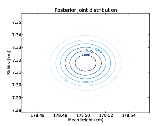
Figure 10.2: Contour plot of the posterior joint distribution of mean and standard deviation of height for women in the U.S.

---

We are almost ready to look at results, but we have one more problem to deal with. There are a number of outliers in this dataset that are almost certainly errors. For example, there are three adults with reported height of 61 cm, which would place them among the shortest living adults in the world. At the other end, there are four women with reported height 229 cm, just short of the tallest women in the world.

It is not impossible that these values are correct, but it is unlikely, which makes it hard to know how to deal with them. But since we are trying to estimate variability, we have to get it right, since these extreme values have a disproportionate effect on the estimates.

Because ABC is based on summary statistics, rather than the entire data set, we can make it more robust by choosing summary statistics that are robust in the presence of outliers. Specifically, rather than use the sample mean and standard deviation, we can use the median and an inter-percentile range. For example, the inter-quartile range (IQR) is the difference between the 25th and 75th percentiles.

More generally, we can compute an inter-percentile range that spans a given fraction of the distribution, p:

def MedianIPR(xs, p=0.6827):
    cdf = thinkbayes.MakeCdfFromList(xs)
    median = cdf.Percentile(50)

    alpha = (1-p) / 2
    ipr = cdf.Value(1-alpha) - cdf.Value(alpha)
    return median, ipr

The result is the median and the inter-percentile range. We can convert from ipr to an estimate of sigma using the Gaussian CDF to compute the fraction of the distribution covered by a given number of standard deviations. For example, it is a well-known rule of thumb that 68% of a Gaussian distribution falls within one standard deviation of the mean, which leaves 16% in each tail. If we compute the range between the 16th and 84th percentiles, we expect the result to be 2 * sigma. So we can estimate sigma by computing the 68% IPR and dividing by 2.

The following function does the same computation for any number of sigmas:

def MedianSighat(xs, num_sigmas):
    half_p = thinkbayes.StandardGaussianCdf(num_sigmas) - 0.5

    median, ipr = MedianIPR(xs, half_p * 2)
    sighat = ipr / 2 / num_sigmas

    return median, sighat

The result is an estimate of sigma, which I call sighat because “hat” is the conventional symbol that indicates an estimate.

Then in LogUpdateSetABC we can replace the conventional estimators, xbar and S, with median and sighat. And that pretty much does it.

It might seem odd that we are using observed percentiles to estimate mu and sigma, but it is an example of the flexibility of the Bayesian approach. In effect we are asking, “Given hypothetical values for mu and sigma, and a sampling process that has some chance of introducing errors, what is the likelihood of generating a given set of sample statistics?”

We are free to choose any sample statistics we like, up to a point: mu and sigma determine the location and spread of a distribution, so we need to choose statistics that capture those characteristics. For example, if we chose the 49th and 51st percentiles, we would get very little information about spread, so it would leave the estimate of sigma relatively unconstrained by the data. All values of sigma would have nearly the same likelihood of producing the observed values, so the posterior marginal distribution for sigma would look a lot like the prior.

10.9  Who is more variable?

---

Figure 10.3: Contour plot of the posterior joint distribution of mean and standard deviation of height for women in the U.S.

---

Finally we are ready to answer the question we started with: is the coefficient of variation greater for men than for women?

Using ABC based on the median and IPR with num_sigmas=1, I computed posterior joint distributions for mu and sigma. Figures 10.1 and  10.2 show the results as a contour plot with mu on the x-axis, sigma on the y-axis, and probability on the z-axis.

The most likely values for men are 178 cm and 7.4 cm, so the maximum likelihood estimate for sigma, based on robust sample statistics, is a bit less than the observed standard deviation, 7.7 cm.

For women, the most likely values are 163 cm and 7.0 cm. Again, the estimate of sigma is less than the observed standard deviation, 7.3 cm.

For each joint distribution, we compute the posterior distribution of CV. Figure 10.3 shows these distributions for men and women. The mean for men is 0.0410; for women it is 0.0429. And since there is no overlap between the distributions, we conclude that women are more variable in height than men.

So is that the end of the Variability Hypothesis? Sadly, no. This result turns out to depend strongly on the choice of the inter-percentile range. With num_sigmas=1, we conclude that women are more variable, but with num_sigmas=2 we conclude with equal confidence that men are more variable.

The reason for the difference is that there are differences in the shapes of the distributions for men and women. Specifically, there are more men of short stature, and their distance from the mean is greater.

So our evaluation of the Variability Hypothesis depends on the interpretation of “variability.” With num_sigmas=1 we are measuring differences between people within one standard deviation of the mean, people we would call “normal” for want of less value-laden word. As we increase num_sigmas, the measure of variability is influenced by an increasing number of people whose stature is affected by medical conditions. How much effect these people should have on the result depends on what notion of variability we are trying to capture, which depends on theory we are trying to test.

In the case of the Variability Hypothesis, I don’t think the theory is sufficiently well-defined to test, and even if it were, I don’t think the results would mean very much.

I hope you agree that this example is interesting, and it helped me demonstrate several new ideas, but at this point we have probably given the Variability Hypothesis more energy than it deserves, so let’s stop there.

You can download the code in this chapter from http://thinkbayes.com/variability.py.

10.10  Exercises

Are you using one of our books in a class?