This HTML version of "Think Stats 2e" is provided for convenience, but it is not the best format for the book. In particular, some of the math symbols are not rendered correctly.

You might prefer to read the PDF version, or you can buy a hard copy from Amazon.

Chapter 7 Relationships between variables

So far we have only looked at one variable at a time. In this chapter we look at relationships between variables. Two variables are related if knowing one gives you information about the other. For example, height and weight are related; people who are taller tend to be heavier. Of course, it is not a perfect relationship: there are short heavy people and tall light ones. But if you are trying to guess someone’s weight, you will be more accurate if you know their height than if you don’t.

The code for this chapter is in scatter.py. For information about downloading and working with this code, see Section 0.2.

7.1 Scatter plots

The simplest way to check for a relationship between two variables is a scatter plot, but making a good scatter plot is not always easy. As an example, I’ll plot weight versus height for the respondents in the BRFSS (see Section 5.4).

Here’s the code that reads the data file and extracts height and weight:

    df = brfss.ReadBrfss(nrows=None)
    sample = thinkstats2.SampleRows(df, 5000)
    heights, weights = sample.htm3, sample.wtkg2

SampleRows chooses a random subset of the data:

def SampleRows(df, nrows, replace=False):
    indices = np.random.choice(df.index, nrows, replace=replace)
    sample = df.loc[indices]
    return sample

df is the DataFrame, nrows is the number of rows to choose, and replace is a boolean indicating whether sampling should be done with replacement; in other words, whether the same row could be chosen more than once.

thinkplot provides Scatter, which makes scatter plots:

    thinkplot.Scatter(heights, weights)
    thinkplot.Show(xlabel='Height (cm)',
                   ylabel='Weight (kg)',
                   axis=[140, 210, 20, 200])

The result, in Figure 7.1 (left), shows the shape of the relationship. As we expected, taller people tend to be heavier.

Figure 7.1: Scatter plots of weight versus height for the respondents in the BRFSS, unjittered (left), jittered (right).

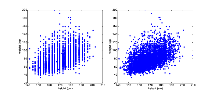
But this is not the best representation of the data, because the data are packed into columns. The problem is that the heights are rounded to the nearest inch, converted to centimeters, and then rounded again. Some information is lost in translation.

We can’t get that information back, but we can minimize the effect on the scatter plot by jittering the data, which means adding random noise to reverse the effect of rounding off. Since these measurements were rounded to the nearest inch, they might be off by up to 0.5 inches or 1.3 cm. Similarly, the weights might be off by 0.5 kg.

    heights = thinkstats2.Jitter(heights, 1.3)
    weights = thinkstats2.Jitter(weights, 0.5)

Here’s the implementation of Jitter:

def Jitter(values, jitter=0.5):
    n = len(values)
    return np.random.uniform(-jitter, +jitter, n) + values

The values can be any sequence; the result is a NumPy array.

Figure 7.1 (right) shows the result. Jittering reduces the visual effect of rounding and makes the shape of the relationship clearer. But in general you should only jitter data for purposes of visualization and avoid using jittered data for analysis.

Even with jittering, this is not the best way to represent the data. There are many overlapping points, which hides data in the dense parts of the figure and gives disproportionate emphasis to outliers. This effect is called saturation.

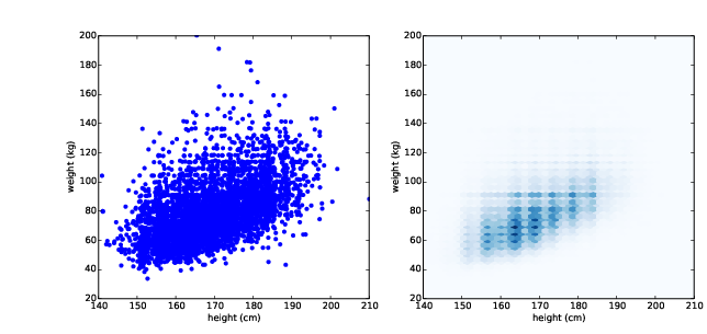
Figure 7.2: Scatter plot with jittering and transparency (left), hexbin plot (right).

We can solve this problem with the alpha parameter, which makes the points partly transparent:

    thinkplot.Scatter(heights, weights, alpha=0.2)

Figure 7.2 (left) shows the result. Overlapping data points look darker, so darkness is proportional to density. In this version of the plot we can see two details that were not apparent before: vertical clusters at several heights and a horizontal line near 90 kg or 200 pounds. Since this data is based on self-reports in pounds, the most likely explanation is that some respondents reported rounded values.

Using transparency works well for moderate-sized datasets, but this figure only shows the first 5000 records in the BRFSS, out of a total of 414 509.

To handle larger datasets, another option is a hexbin plot, which divides the graph into hexagonal bins and colors each bin according to how many data points fall in it. thinkplot provides HexBin:

    thinkplot.HexBin(heights, weights)

Figure 7.2 (right) shows the result. An advantage of a hexbin is that it shows the shape of the relationship well, and it is efficient for large datasets, both in time and in the size of the file it generates. A drawback is that it makes the outliers invisible.

The point of this example is that it is not easy to make a scatter plot that shows relationships clearly without introducing misleading artifacts.

7.2 Characterizing relationships

Scatter plots provide a general impression of the relationship between variables, but there are other visualizations that provide more insight into the nature of the relationship. One option is to bin one variable and plot percentiles of the other.

NumPy and pandas provide functions for binning data:

    df = df.dropna(subset=['htm3', 'wtkg2'])
    bins = np.arange(135, 210, 5)
    indices = np.digitize(df.htm3, bins)
    groups = df.groupby(indices)

dropna drops rows with nan in any of the listed columns. arange makes a NumPy array of bins from 135 to, but not including, 210, in increments of 5.

digitize computes the index of the bin that contains each value in df.htm3. The result is a NumPy array of integer indices. Values that fall below the lowest bin are mapped to index 0. Values above the highest bin are mapped to len(bins).

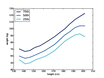
Figure 7.3: Percentiles of weight for a range of height bins.

groupby is a DataFrame method that returns a GroupBy object; used in a for loop, groups iterates the names of the groups and the DataFrames that represent them. So, for example, we can print the number of rows in each group like this:

for i, group in groups:
    print(i, len(group))

Now for each group we can compute the mean height and the CDF of weight:

    heights = [group.htm3.mean() for i, group in groups]
    cdfs = [thinkstats2.Cdf(group.wtkg2) for i, group in groups]

Finally, we can plot percentiles of weight versus height:

    for percent in [75, 50, 25]:
        weights = [cdf.Percentile(percent) for cdf in cdfs]
        label = '%dth' % percent
        thinkplot.Plot(heights, weights, label=label)

Figure 7.3 shows the result. Between 140 and 200 cm the relationship between these variables is roughly linear. This range includes more than 99% of the data, so we don’t have to worry too much about the extremes.

7.3 Correlation

A correlation is a statistic intended to quantify the strength of the relationship between two variables.

A challenge in measuring correlation is that the variables we want to compare are often not expressed in the same units. And even if they are in the same units, they come from different distributions.

There are two common solutions to these problems:

Transform each value to a standard score, which is the number of standard deviations from the mean. This transform leads to the “Pearson product-moment correlation coefficient.”
Transform each value to its rank, which is its index in the sorted list of values. This transform leads to the “Spearman rank correlation coefficient.”

If X is a series of n values, x_i, we can convert to standard scores by subtracting the mean and dividing by the standard deviation: z_i = (x_i − µ) / σ.

The numerator is a deviation: the distance from the mean. Dividing by σ standardizes the deviation, so the values of Z are dimensionless (no units) and their distribution has mean 0 and variance 1.

If X is normally distributed, so is Z. But if X is skewed or has outliers, so does Z; in those cases, it is more robust to use percentile ranks. If we compute a new variable, R, so that r_i is the rank of x_i, the distribution of R is uniform from 1 to n, regardless of the distribution of X.

7.4 Covariance

Covariance is a measure of the tendency of two variables to vary together. If we have two series, X and Y, their deviations from the mean are

dx_i = x_i − x

dy_i = y_i − ȳ

where x is the sample mean of X and ȳ is the sample mean of Y. If X and Y vary together, their deviations tend to have the same sign.

If we multiply them together, the product is positive when the deviations have the same sign and negative when they have the opposite sign. So adding up the products gives a measure of the tendency to vary together.

Covariance is the mean of these products:

Cov(X,Y) =

∑dx_i dy_i

where n is the length of the two series (they have to be the same length).

If you have studied linear algebra, you might recognize that Cov is the dot product of the deviations, divided by their length. So the covariance is maximized if the two vectors are identical, 0 if they are orthogonal, and negative if they point in opposite directions. thinkstats2 uses np.dot to implement Cov efficiently:

def Cov(xs, ys, meanx=None, meany=None):
    xs = np.asarray(xs)
    ys = np.asarray(ys)

    if meanx is None:
        meanx = np.mean(xs)
    if meany is None:
        meany = np.mean(ys)

    cov = np.dot(xs-meanx, ys-meany) / len(xs)
    return cov

By default Cov computes deviations from the sample means, or you can provide known means. If xs and ys are Python sequences, np.asarray converts them to NumPy arrays. If they are already NumPy arrays, np.asarray does nothing.

This implementation of covariance is meant to be simple for purposes of explanation. NumPy and pandas also provide implementations of covariance, but both of them apply a correction for small sample sizes that we have not covered yet, and np.cov returns a covariance matrix, which is more than we need for now.

7.5 Pearson’s correlation

Covariance is useful in some computations, but it is seldom reported as a summary statistic because it is hard to interpret. Among other problems, its units are the product of the units of X and Y. For example, the covariance of weight and height in the BRFSS dataset is 113 kilogram-centimeters, whatever that means.

One solution to this problem is to divide the deviations by the standard deviation, which yields standard scores, and compute the product of standard scores:

p_i =

(x_i − x)

S_X

(y_i − ȳ)

S_Y

Where S_X and S_Y are the standard deviations of X and Y. The mean of these products is

ρ =

∑p_i

Or we can rewrite ρ by factoring out S_X and S_Y:

ρ =

Cov(X,Y)

S_X S_Y

This value is called Pearson’s correlation after Karl Pearson, an influential early statistician. It is easy to compute and easy to interpret. Because standard scores are dimensionless, so is ρ.

Here is the implementation in thinkstats2:

def Corr(xs, ys):
    xs = np.asarray(xs)
    ys = np.asarray(ys)

    meanx, varx = MeanVar(xs)
    meany, vary = MeanVar(ys)

    corr = Cov(xs, ys, meanx, meany) / math.sqrt(varx * vary)
    return corr

MeanVar computes mean and variance slightly more efficiently than separate calls to np.mean and np.var.

Pearson’s correlation is always between -1 and +1 (including both). If ρ is positive, we say that the correlation is positive, which means that when one variable is high, the other tends to be high. If ρ is negative, the correlation is negative, so when one variable is high, the other is low.

The magnitude of ρ indicates the strength of the correlation. If ρ is 1 or -1, the variables are perfectly correlated, which means that if you know one, you can make a perfect prediction about the other.

Most correlation in the real world is not perfect, but it is still useful. The correlation of height and weight is 0.51, which is a strong correlation compared to similar human-related variables.

7.6 Nonlinear relationships

If Pearson’s correlation is near 0, it is tempting to conclude that there is no relationship between the variables, but that conclusion is not valid. Pearson’s correlation only measures linear relationships. If there’s a nonlinear relationship, ρ understates its strength.

Figure 7.4: Examples of datasets with a range of correlations.

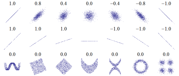
Figure 7.4 is from http://wikipedia.org/wiki/Correlation_and_dependence. It shows scatter plots and correlation coefficients for several carefully constructed datasets.

The top row shows linear relationships with a range of correlations; you can use this row to get a sense of what different values of ρ look like. The second row shows perfect correlations with a range of slopes, which demonstrates that correlation is unrelated to slope (we’ll talk about estimating slope soon). The third row shows variables that are clearly related, but because the relationship is nonlinear, the correlation coefficient is 0.

The moral of this story is that you should always look at a scatter plot of your data before blindly computing a correlation coefficient.

7.7 Spearman’s rank correlation

Pearson’s correlation works well if the relationship between variables is linear and if the variables are roughly normal. But it is not robust in the presence of outliers. Spearman’s rank correlation is an alternative that mitigates the effect of outliers and skewed distributions. To compute Spearman’s correlation, we have to compute the rank of each value, which is its index in the sorted sample. For example, in the sample [1, 2, 5, 7] the rank of the value 5 is 3, because it appears third in the sorted list. Then we compute Pearson’s correlation for the ranks.

thinkstats2 provides a function that computes Spearman’s rank correlation:

def SpearmanCorr(xs, ys):
    xranks = pandas.Series(xs).rank()
    yranks = pandas.Series(ys).rank()
    return Corr(xranks, yranks)

I convert the arguments to pandas Series objects so I can use rank, which computes the rank for each value and returns a Series. Then I use Corr to compute the correlation of the ranks.

I could also use Series.corr directly and specify Spearman’s method:

def SpearmanCorr(xs, ys):
    xs = pandas.Series(xs)
    ys = pandas.Series(ys)
    return xs.corr(ys, method='spearman')

The Spearman rank correlation for the BRFSS data is 0.54, a little higher than the Pearson correlation, 0.51. There are several possible reasons for the difference, including:

If the relationship is nonlinear, Pearson’s correlation tends to underestimate the strength of the relationship, and
Pearson’s correlation can be affected (in either direction) if one of the distributions is skewed or contains outliers. Spearman’s rank correlation is more robust.

In the BRFSS example, we know that the distribution of weights is roughly lognormal; under a log transform it approximates a normal distribution, so it has no skew. So another way to eliminate the effect of skewness is to compute Pearson’s correlation with log-weight and height:

    thinkstats2.Corr(df.htm3, np.log(df.wtkg2))

The result is 0.53, close to the rank correlation, 0.54. So that suggests that skewness in the distribution of weight explains most of the difference between Pearson’s and Spearman’s correlation.

7.8 Correlation and causation

If variables A and B are correlated, there are three possible explanations: A causes B, or B causes A, or some other set of factors causes both A and B. These explanations are called “causal relationships”.

Correlation alone does not distinguish between these explanations, so it does not tell you which ones are true. This rule is often summarized with the phrase “Correlation does not imply causation,” which is so pithy it has its own Wikipedia page: http://wikipedia.org/wiki/Correlation_does_not_imply_causation.

So what can you do to provide evidence of causation?

Use time. If A comes before B, then A can cause B but not the other way around (at least according to our common understanding of causation). The order of events can help us infer the direction of causation, but it does not preclude the possibility that something else causes both A and B.
Use randomness. If you divide a large sample into two groups at random and compute the means of almost any variable, you expect the difference to be small. If the groups are nearly identical in all variables but one, you can eliminate spurious relationships.
This works even if you don’t know what the relevant variables are, but it works even better if you do, because you can check that the groups are identical.

These ideas are the motivation for the randomized controlled trial, in which subjects are assigned randomly to two (or more) groups: a treatment group that receives some kind of intervention, like a new medicine, and a control group that receives no intervention, or another treatment whose effects are known.

A randomized controlled trial is the most reliable way to demonstrate a causal relationship, and the foundation of science-based medicine (see http://wikipedia.org/wiki/Randomized_controlled_trial).

Unfortunately, controlled trials are only possible in the laboratory sciences, medicine, and a few other disciplines. In the social sciences, controlled experiments are rare, usually because they are impossible or unethical.

An alternative is to look for a natural experiment, where different “treatments” are applied to groups that are otherwise similar. One danger of natural experiments is that the groups might differ in ways that are not apparent. You can read more about this topic at http://wikipedia.org/wiki/Natural_experiment.

In some cases it is possible to infer causal relationships using regression analysis, which is the topic of Chapter 11.

7.9 Exercises

A solution to this exercise is in chap07soln.py.

Exercise 1 Using data from the NSFG, make a scatter plot of birth weight versus mother’s age. Plot percentiles of birth weight versus mother’s age. Compute Pearson’s and Spearman’s correlations. How would you characterize the relationship between these variables?

7.10 Glossary

scatter plot: A visualization of the relationship between two variables, showing one point for each row of data.
jitter: Random noise added to data for purposes of visualization.
saturation: Loss of information when multiple points are plotted on top of each other.
correlation: A statistic that measures the strength of the relationship between two variables.
standardize: To transform a set of values so that their mean is 0 and their variance is 1.
standard score: A value that has been standardized so that it is expressed in standard deviations from the mean.
covariance: A measure of the tendency of two variables to vary together.
rank: The index where an element appears in a sorted list.
randomized controlled trial: An experimental design in which subjects are divided into groups at random, and different groups are given different treatments.
treatment group: A group in a controlled trial that receives some kind of intervention.
control group: A group in a controlled trial that receives no treatment, or a treatment whose effect is known.
natural experiment: An experimental design that takes advantage of a natural division of subjects into groups in ways that are at least approximately random.