Chapter 6 Cellular AutomataA cellular automaton is a model of a world with very simple physics. “Cellular” means that the space is divided into discrete chunks, called cells. An “automaton” is a machine that performs computations—it could be a real machine, but more often the “machine” is a mathematical abstraction or a computer simulation. Automata are governed by rules that determine how the system evolves in time. Time is divided into discrete steps, and the rules specify how to compute the state of the world during the next time step based on the current state. As a trivial example, consider a cellular automaton (CA) with a single cell. The state of the cell is an integer represented with the variable xi, where the subscript i indicates that xi is the state of the system during time step i. As an initial condition, x0 = 0. Now all we need is a rule. Arbitrarily, I’ll pick xi = xi−1 + 1, which says that after each time step, the state of the CA gets incremented by 1. So far, we have a simple CA that performs a simple calculation: it counts. But this CA is atypical; normally the number of possible states is finite. To bring it into line, I’ll choose the smallest interesting number of states, 2, and another simple rule, xi = (xi−1 + 1) % 2, where % is the remainder (or modulus) operator. This CA performs a simple calculation: it blinks. That is, the state of the cell switches between 0 and 1 after every time step. Most CAs are deterministic, which means that rules do not have any random elements; given the same initial state, they always produce the same result. There are also nondeterministic CAs, but I will not address them here. 6.1 Stephen WolframThe CA in the previous section was 0-dimensional and it wasn’t very interesting. But 1-dimensional CAs turn out to be surprisingly interesting. In the early 1980s Stephen Wolfram published a series of papers presenting a systematic study of 1-dimensional CAs. He identified four general categories of behavior, each more interesting than the last. To say that a CA has dimensions is to say that the cells are arranged in a contiguous space so that some of them are considered “neighbors.” In one dimension, there are three natural configurations:
The rules that determine how the system evolves in time are based on the notion of a “neighborhood,” which is the set of cells that determines the next state of a given cell. Wolfram’s experiments use a 3-cell neighborhood: the cell itself and its left and right neighbors. In these experiments, the cells have two states, denoted 0 and 1, so the rules can be summarized by a table that maps from the state of the neighborhood (a tuple of 3 states) to the next state for the center cell. The following table shows an example:
The row first shows the eight states a neighborhood can be in. The second row shows the state of the center cell during the next time step. As a concise encoding of this table, Wolfram suggested reading the bottom row as a binary number. Because 00110010 in binary is 50 in decimal, Wolfram calls this CA “Rule 50.” Figure 6.1 shows the effect of Rule 50 over 10 time steps. The first row shows the state of the system during the first time step; it starts with one cell “on” and the rest “off”. The second row shows the state of the system during the next time step, and so on. The triangular shape in the figure is typical of these CAs; is it a consequence of the shape of the neighborhood. In one time step, each cell influences the state of one neighbor in either direction. During the next time step, that influence can propagate one more cell in each direction. So each cell in the past has a “triangle of influence” that includes all of the cells that can be affected by it. 6.2 Implementing CAsTo generate the previous figure, I wrote a Python program that implements and draws CAs. You can download my code from thinkcomplex.com/CA.py. and thinkcomplex.com/CADrawer.py. To store the state of the CA, I use a NumPy array. An array is a multi-dimensional data structure whose elements are all the same type. It is similar to a nested list, but usually smaller and faster. Figure 6.2 shows why. The diagram on the left shows a list of lists of integers; each dot represents a reference, which takes up 4–8 bytes. To access one of the integers, you have to follow two references. The diagram on the right shows an array of the same integers. Because the elements are all the same size, they can be stored contiguously in memory. This arrangement saves space because it doesn’t use references, and it saves time because the location of an element can be computed directly from the indices; there is no need to follow a series of references. Here is a CA object that uses a NumPy array: import numpy
class CA(object):
def __init__(self, rule, n=100, ratio=2):
self.table = make_table(rule)
self.n = n
self.m = ratio*n + 1
self.array = numpy.zeros((n, self.m), dtype=numpy.int8)
self.next = 0
rule is an integer in the range 0-255, which represents the
CA rule table using Wolfram’s encoding. n is the number of rows in the array, which is the number of time steps we will compute. m is the number of columns, which is the number of cells. To get started, I’ll implement a finite array of cells. zeros is provided by NumPy; it creates a new array with the given dimensions, n by m; dtype stands for “data type,” and it specifies the type of the array elements. int8 is an 8-bit integer, so we are limited to 256 states, but that’s no problem: we only need two. next is the index of the next time step. There are two common starting conditions for CAs: a single cell, or a row
of random cells. def start_single(self):
"""Starts with one cell in the middle of the top row."""
self.array[0, self.m/2] = 1
self.next += 1
The array index is a tuple that species the row and column of the cell, in that order. step computes the next state of the CA: def step(self):
i = self.next
self.next += 1
a = self.array
t = self.table
for j in xrange(1,self.m-1):
a[i,j] = t[tuple(a[i-1, j-1:j+2])]
i is the time step and the index of the row we are about to compute. j loops through the cells, skipping the first and last, which are always off. Arrays support slice operations, so self.array[i-1, j-1:j+2] gets three elements from row i-1. Then we look up the neighborhood tuple in the table, get the next state, and store it in the array. Array indexing is constant time, so step is linear in n. Filling in the whole array is O(nm). You can read more about NumPy and arrays at scipy.org/Tentative_NumPy_Tutorial. 6.3 CADrawerAn abstract class is a class definition that specifies the interface for a set of methods without providing an implementation. Child classes extend the abstract class and implement the incomplete methods. See http://en.wikipedia.org/wiki/Abstract_type. As an example, CADrawer defines an interface for drawing CAs; here is the definition: class Drawer(object):
"""Drawer is an abstract class that should not be instantiated.
It defines the interface for a CA drawer; child classes of Drawer
should implement draw, show and save.
If draw_array is not overridden, the child class should provide
draw_cell.
"""
def __init__(self):
msg = 'CADrawer is an abstract type and should not be instantiated.'
raise UnimplementedMethodException, msg
def draw(self, ca):
"""Draws a representation of cellular automaton (CA).
This function generally has no visible effect."""
raise UnimplementedMethodException
def draw_array(self, a):
"""Iterate through array (a) and draws any non-zero cells."""
for i in xrange(self.rows):
for j in xrange(self.cols):
if a[i,j]:
self.draw_cell(j, self.rows-i-1)
def draw_cell(self, ca):
"""Draws a single cell.
Not required for all implementations."""
raise UnimplementedMethodException
def show(self):
"""Displays the representation on the screen, if possible."""
raise UnimplementedMethodException
def save(self, filename):
"""Saves the representation of the CA in filename."""
raise UnimplementedMethodException
Abstract classes should not be instantiated; if you try, you get an UnimplementedMethodException, which is a simple extension of Exception: class UnimplementedMethodException(Exception):
"""Used to indicate that a child class has not implemented an
abstract method."""
To instantiate a CADrawer you have to define a child class that implements the methods, then instantiate the child. CADrawer.py provides three implementations, one that uses pyplot, one that uses the Python Imaging Library (PIL), and one that generates Encapsulated Postscript (EPS). Here is an example that uses PyplotDrawer to display a CA on the screen: ca = CA(rule, n)
ca.start_single()
ca.loop(n-1)
drawer = CADrawer.PyplotDrawer()
drawer.draw(ca)
drawer.show()
Exercise 1 Download thinkcomplex.com/CA.py and thinkcomplex.com/CADrawer.py and confirm that they run on your system; you might have to install additional Python packages. Create a new class called CircularCA that extends CA so that the cells are arranged in a ring. Hint: you might find it useful to add a column of “ghost cells” to the array. You can download my solution from thinkcomplex.com/CircularCA.py 6.4 Classifying CAsWolfram proposes that the behavior of CAs can be grouped into four classes. Class 1 contains the simplest (and least interesting) CAs, the ones that evolve from almost any starting condition to the same uniform pattern. As a trivial example, Rule 0 always generates an empty pattern after one time step. Rule 50 is an example of Class 2. It generates a simple pattern with nested structure; that is, the pattern contains many smaller versions of itself. Rule 18 makes the nested structure even clearer; Figure 6.3 shows what it looks like after 64 steps. This pattern resembles the Sierpiński triangle, which you can read about at http://en.wikipedia.org/wiki/Sierpinski_triangle. Some Class 2 CAs generate patterns that are intricate and pretty, but compared to Classes 3 and 4, they are relatively simple. 6.5 RandomnessClass 3 contains CAs that generate randomness. Rule 30 is an example; Figure 6.4 shows what it looks like after 100 time steps. Along the left side there is an apparent pattern, and on the right side there are triangles in various sizes, but the center seems quite random. In fact, if you take the center column and treat it as a sequence of bits, it is hard to distinguish from a truly random sequence. It passes many of the statistical tests people use to test whether a sequence of bits is random. Programs that produce random-seeming numbers are called pseudo-random number generators (PRNGs). They are not considered truly random because
Modern PRNGs produce sequences that are statistically indistinguishable from random, and they can be implemented with with periods so long that the universe will collapse before they repeat. The existence of these generators raises the question of whether there is any real difference between a good quality pseudo-random sequence and a sequence generated by a “truly” random process. In A New Kind of Science, Wolfram argues that there is not (pages 315–326). Exercise 2 This exercise asks you to implement and test several PRNGs.
6.6 DeterminismThe existence of Class 3 CAs is surprising. To understand how surprising, it is useful to consider philosophical determinism (see http://en.wikipedia.org/wiki/Determinism). Most philosophical stances are hard to define precisely because they come in a variety of flavors. I often find it useful to define them with a list of statements ordered from weak to strong:
My goal in constructing this range is to make D1 so weak that virtually everyone would accept it, D4 so strong that almost no one would accept it, with intermediate statements that some people accept. The center of mass of world opinion swings along this range in response to historical developments and scientific discoveries. Prior to the scientific revolution, many people regarded the working of the universe as fundamentally unpredictable or controlled by supernatural forces. After the triumphs of Newtonian mechanics, some optimists came to believe something like D4; for example, in 1814 Pierre-Simon Laplace wrote We may regard the present state of the universe as the effect of its past and the cause of its future. An intellect which at a certain moment would know all forces that set nature in motion, and all positions of all items of which nature is composed, if this intellect were also vast enough to submit these data to analysis, it would embrace in a single formula the movements of the greatest bodies of the universe and those of the tiniest atom; for such an intellect nothing would be uncertain and the future just like the past would be present before its eyes. This “intellect” came to be called “Laplace’s Demon”. See http://en.wikipedia.org/wiki/Laplace's_demon. The word “demon” in this context has the sense of “spirit,” with no implication of evil. Discoveries in the 19th and 20th centuries gradually dismantled this hope. The thermodynamic concept of entropy, radioactive decay, and quantum mechanics posed successive challenges to strong forms of determinism. In the 1960s chaos theory showed that in some deterministic systems prediction is only possible over short time scales, limited by the precision of measurement of initial conditions. Most of these systems are continuous in space (if not time) and nonlinear, so the complexity of their behavior is not entirely surprising. Wolfram’s demonstration of complex behavior in simple cellular automata is more surprising—and disturbing, at least to a deterministic world view. So far I have focused on scientific challenges to determinism, but the longest-standing objection is the conflict between determinism and human free will. Complexity science provides a possible resolution of this apparent conflict; we come back to this topic in Section 10.7. 6.7 StructuresThe behavior of Class 4 CAs is even more surprising. Several 1-D CAs, most notably Rule 110, are Turing complete, which means that they can compute any computable function. This property, also called universality, was proved by Matthew Cook in 1998. See http://en.wikipedia.org/wiki/Rule_110. Figure 6.5 shows what Rule 110 looks like with an initial condition of a single cell and 100 time steps. At this time scale it is not apparent that anything special is going on. There are some regular patterns but also some features that are hard to characterize. Figure 6.6 shows a bigger picture, starting with a random initial condition and 600 time steps: After about 100 steps the background settles into a simple repeating pattern, but there are a number of persistent structures that appear as disturbances in the background. Some of these structures are stable, so they appear as vertical lines. Others translate in space, appearing as diagonals with different slopes, depending on how many time steps they take to shift by one column. These structures are called spaceships. Collisions between spaceships yield different results depending on the types of the spaceships and the phase they are in when they collide. Some collisions annihilate both ships; others leave one ship unchanged; still others yield one or more ships of different types. These collisions are the basis of computation in a Rule 110 CA. If you think of spaceships as signals that propagate on wires, and collisions as gates that compute logical operations like AND and OR, you can see what it means for a CA to perform a computation. Exercise 3 This exercise asks you to experiment with Rule 110 and see how many spaceships you can find.
6.8 UniversalityTo understand universality, we have to understand computability theory, which is about models of computation and what they compute. One of the most general models of computation is the Turing machine, which is an abstract computer proposed by Alan Turing in 1936. A Turing machine is a 1-D CA, infinite in both directions, augmented with a read-write head. At any time, the head is positioned over a single cell. It can read the state of that cell (usually there are only two states) and it can write a new value into the cell. In addition, the machine has a register, which records the state of the machine (one of a finite number of states), and a table of rules. For each machine state and cell state, the table specifies an action. Actions include modifying the cell the head is over and moving one cell to the left or right. A Turing machine is not a practical design for a computer, but it models common computer architectures. For a given program running on a real computer, it is possible (at least in principle) to construct a Turing machine that performs an equivalent computation. The Turing machine is useful because it is possible to characterize the set of functions that can be computed by a Turing machine, which is what Turing did. Functions in this set are called Turing computable. To say that a Turing machine can compute any Turing-computable function is a tautology: it is true by definition. But Turing-computability is more interesting than that. It turns out that just about every reasonable model of computation anyone has come up with is Turing complete; that is, it can compute exactly the same set of functions as the Turing machine. Some of these models, like lamdba calculus, are very different from a Turing machine, so their equivalence is surprising. This observation led to the Church-Turing Thesis, which is essentially a definition of what it means to be computable. The “thesis” is that Turing-computability is the right, or at least natural, definition of computability, because it describes the power of such a diverse collection of models of computation. The Rule 110 CA is yet another model of computation, and remarkable for its simplicity. That it, too, turns out to be universal lends support to the Church-Turing Thesis. In A New Kind of Science, Wolfram states a variation of this thesis, which he calls the “principle of computational equivalence:” Almost all processes that are not obviously simple can be viewed as computations of equivalent sophistication. Applying these definitions to CAs, Classes 1 and 2 are “obviously simple.” It may be less obvious that Class 3 is simple, but in a way perfect randomness is as simple as perfect order; complexity happens in between. So Wolfram’s claim is that Class 4 behavior is common in the natural world, and that almost all of the systems that manifest it are computationally equivalent. Exercise 4 The goal of this exercise is to implement a Turing machine. See http://en.wikipedia.org/wiki/Turing_machine.
6.9 FalsifiabilityWolfram holds that his principle is a stronger claim than the Church-Turing Thesis because it is about the natural world rather than abstract models of computation. But saying that natural processes “can be viewed as computations” strikes me as a statement about theory choice more than a hypothesis about the natural world. Also, with qualifications like “almost” and undefined terms like “obviously simple,” his hypothesis may be unfalsifiable. Falsifiability is an idea from the philosophy of science, proposed by Karl Popper as a demarcation between scientific hypotheses and pseudoscience. A hypothesis is falsifiable if there is an experiment, at least in the realm of practicality, that would contradict the hypothesis if it were false. For example, the claim that all life on earth is descended from a common ancestor is falsifiable because it makes specific predictions about similarities in the genetics of modern species (among other things). If we discovered a new species whose DNA was almost entirely different from ours, that would contradict (or at least bring into question) the theory of universal common descent. On the other hand, “special creation,” the claim that all species were created in their current form by a supernatural agent, is unfalsifiable because there is nothing that we could observe about the natural world that would contradict it. Any outcome of any experiment could be attributed to the will of the creator. Unfalsifiable hypotheses can be appealing because they are impossible to refute. If your goal is never to be proved wrong, you should choose hypotheses that are as unfalsifiable as possible. But if your goal is to make reliable predictions about the world—and this is at least one of the goals of science—then unfalsifiable hypotheses are useless. The problem is that they have no consequences (if they had consequences, they would be falsifiable). For example, if the theory of special creation were true, what good would it do me to know it? It wouldn’t tell me anything about the creator except that he has an “inordinate fondness for beetles” (attributed to J. B. S. Haldane). And unlike the theory of common descent, which informs many areas of science and bioengineering, it would be of no use for understanding the world or acting in it. Exercise 5 Falsifiability is an appealing and useful idea, but among philosophers of science it is not generally accepted as a solution to the demarcation problem, as Popper claimed. Read http://en.wikipedia.org/wiki/Falsifiability and answer the following questions.
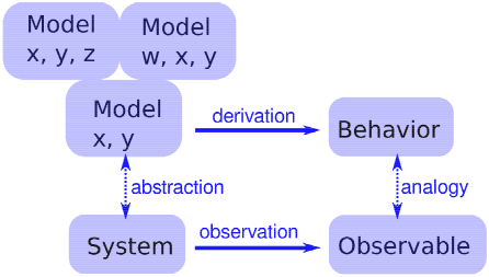
6.10 What is this a model of?Some cellular automata are primarily mathematical artifacts. They are interesting because they are surprising, or useful, or pretty, or because they provide tools for creating new mathematics (like the Church-Turing thesis). But it is not clear that they are models of physical systems. And if they are, they are highly abstracted, which is to say that they are not very detailed or realistic. For example, some species of cone snail produce a pattern on their shells that resembles the patterns generated by cellular automata (seee en.wikipedia.org/wiki/Cone_snail). So it is natural to suppose that a CA is a model of the mechanism that produces patterns on shells as they grow. But, at least initially, it is not clear how the elements of the model (so-called cells, communication between neighbors, rules) correspond to the elements of a growing snail (real cells, chemical signals, protein interaction networks). For conventional physical models, being realistic is a virtue, at least up to a point. If the elements of a model correspond to the elements of a physical system, there is an obvious analogy between the model and the system. In general, we expect a model that is more realistic to make better predictions and to provide more believable explanations. Of course, this is only true up to a point. Models that are more detailed are harder to work with, and usually less amenable to analysis. At some point, a model becomes so complex that it is easier to experiment with the system. At the other extreme, simple models can be compelling exactly because they are simple. Simple models offer a different kind of explanation than detailed models. With a detailed model, the argument goes something like this: “We are interested in physical system S, so we construct a detailed model, M, and show by analysis and simulation that M exhibits a behavior, B, that is similar (qualitatively or quantitatively) to an observation of the real system, O. So why does O happen? Because S is similar to M, and B is similar to O, and we can prove that M leads to B.” With simple models we can’t claim that S is similar to M, because it isn’t. Instead, the argument goes like this: “There is a set of models that share a common set of features. Any model that has these features exhibits behavior B. If we make an observation, O, that resembles B, one way to explain it is to show that the system, S, has the set of features sufficient to produce B.” For this kind of argument, adding more features doesn’t help. Making the model more realistic doesn’t make the model more reliable; it only obscures the difference between the essential features that cause O and the incidental features that are particular to S. Figure 6.7 shows the logical structure of this kind of model. The features x and y are sufficient to produce the behavior. Adding more detail, like features w and z, might make the model more realistic, but that realism adds no explanatory power. |
Like this book?
Are you using one of our books in a class?We'd like to know about it. Please consider filling out this short survey.
|