


This HTML version of
You might prefer to read the PDF version, or you can buy a hard copy from Amazon.
Chapter 6 Decision Analysis
6.1 The Price is Right problem
On November 1, 2007, contestants named Letia and Nathaniel appeared on The Price is Right, an American game show. They competed in a game called The Showcase, where the objective is to guess the price of a showcase of prizes. The contestant who comes closest to the actual price of the showcase, without going over, wins the prizes.
Nathaniel went first. His showcase included a dishwasher, a wine cabinet, a laptop computer, and a car. He bid $26,000.
Letia’s showcase included a pinball machine, a video arcade game, a pool table, and a cruise of the Bahamas. She bid $21,500.
The actual price of Nathaniel’s showcase was $25,347. His bid was too high, so he lost.
The actual price of Letia’s showcase was $21,578. She was only off by $78, so she won her showcase and, because her bid was off by less than $250, she also won Nathaniel’s showcase.
For a Bayesian thinker, this scenario suggests several questions:
- Before seeing the prizes, what prior beliefs should the contestant have about the price of the showcase?
- After seeing the prizes, how should the contestant update those beliefs?
- Based on the posterior distribution, what should the contestant bid?
The third question demonstrates a common use of Bayesian analysis: decision analysis. Given a posterior distribution, we can choose the bid that maximizes the contestant’s expected return.
This problem is inspired by an example in Cameron Davidson-Pilon’s book, Bayesian Methods for Hackers. The code I wrote for this chapter is available from http://thinkbayes.com/price.py; it reads data files you can download from http://thinkbayes.com/showcases.2011.csv and http://thinkbayes.com/showcases.2012.csv. For more information see Section 0.3.
6.2 The prior
Figure 6.1: Distribution of prices for showcases on The Price is Right, 2011-12.
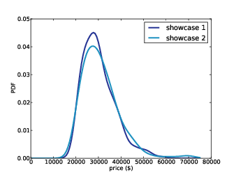
To choose a prior distribution of prices, we can take advantage of data from previous episodes. Fortunately, fans of the show keep detailed records. When I corresponded with Mr. Davidson-Pilon about his book, he sent me data collected by Steve Gee at http://tpirsummaries.8m.com. It includes the price of each showcase from the 2011 and 2012 seasons and the bids offered by the contestants.
Figure 6.1 shows the distribution of prices for these showcases. The most common value for both showcases is around $28,000, but the first showcase has a second mode near $50,000, and the second showcase is occasionally worth more than $70,000.
These distributions are based on actual data, but they have been smoothed by Gaussian kernel density estimation (KDE). Before we go on, I want to take a detour to talk about probability density functions and KDE.
6.3 Probability density functions
So far we have been working with probability mass functions, or PMFs. A PMF is a map from each possible value to its probability. In my implementation, a Pmf object provides a method named Prob that takes a value and returns a probability, also known as a probability mass.
A probability density function, or PDF, is the continuous version of a PMF, where the possible values make up a continuous range rather than a discrete set.
In mathematical notation, PDFs are usually written as functions; for example, here is the PDF of a Gaussian distribution with mean 0 and standard deviation 1:
| f(x) = |
| exp(−x2/2) |
For a given value of x, this function computes a probability density. A density is similar to a probability mass in the sense that a higher density indicates that a value is more likely.
But a density is not a probability. A density can be 0 or any positive value; it is not bounded, like a probability, between 0 and 1.
If you integrate a density over a continuous range, the result is a probability. But for the applications in this book we seldom have to do that.
Instead we primarily use probability densities as part of a likelihood function. We will see an example soon.
6.4 Representing PDFs
To represent PDFs in Python, thinkbayes.py provides a class named Pdf. Pdf is an abstract type, which means that it defines the interface a Pdf is supposed to have, but does not provide a complete implementation. The Pdf interface includes two methods, Density and MakePmf:
class Pdf(object):

    def Density(self, x):
        raise UnimplementedMethodException()

    def MakePmf(self, xs):
        pmf = Pmf()
        for x in xs:
            pmf.Set(x, self.Density(x))
        pmf.Normalize()
        return pmf
Density takes a value, x, and returns the corresponding density. MakePmf makes a discrete approximation to the PDF.
Pdf provides an implementation of MakePmf, but not Density, which has to be provided by a child class.
A concrete type is a child class that extends an abstract type and provides an implementation of the missing methods. For example, GaussianPdf extends Pdf and provides Density:
class GaussianPdf(Pdf):

    def __init__(self, mu, sigma):
        self.mu = mu
        self.sigma = sigma

    def Density(self, x):
        return scipy.stats.norm.pdf(x, self.mu, self.sigma)
__init__ takes mu and sigma, which are
the mean and standard deviation of the distribution, and stores
them as attributes.
Density uses a function from scipy.stats to evaluate the Gaussian PDF. The function is called norm.pdf because the Gaussian distribution is also called the “normal” distribution.
The Gaussian PDF is defined by a simple mathematical function, so it is easy to evaluate. And it is useful because many quantities in the real world have distributions that are approximately Gaussian.
But with real data, there is no guarantee that the distribution is Gaussian or any other simple mathematical function. In that case we can use a sample to estimate the PDF of the whole population.
For example, in The Price Is Right data, we have 313 prices for the first showcase. We can think of these values as a sample from the population of all possible showcase prices.
This sample includes the following values (in order):
| 28800, 28868, 28941, 28957, 28958 |
In the sample, no values appear between 28801 and 28867, but there is no reason to think that these values are impossible. Based on our background information, we expect all values in this range to be equally likely. In other words, we expect the PDF to be fairly smooth.
Kernel density estimation (KDE) is an algorithm that takes a sample and finds an appropriately smooth PDF that fits the data. You can read details at http://en.wikipedia.org/wiki/Kernel_density_estimation.
scipy provides an implementation of KDE and thinkbayes provides a class called EstimatedPdf that uses it:
class EstimatedPdf(Pdf):

    def __init__(self, sample):
        self.kde = scipy.stats.gaussian_kde(sample)

    def Density(self, x):
        return self.kde.evaluate(x)
__init__ takes a sample
and computes a kernel density estimate. The result is a
gaussian_kde object that provides an evaluate
method.
Density takes a value, calls gaussian_kde.evaluate,
and returns the resulting density.
Finally, here’s an outline of the code I used to generate Figure 6.1:
    prices = ReadData()
    pdf = thinkbayes.EstimatedPdf(prices)

    low, high = 0, 75000
    n = 101
    xs = numpy.linspace(low, high, n)
    pmf = pdf.MakePmf(xs)
pdf is a Pdf object, estimated by KDE. pmf is a Pmf object that approximates the Pdf by evaluating the density at a sequence of equally spaced values.
linspace stands for “linear space.” It takes a range, low and high, and the number of points, n, and returns a new numpy array with n elements equally spaced between low and high, including both.
And now back to The Price is Right.
6.5 Modeling the contestants
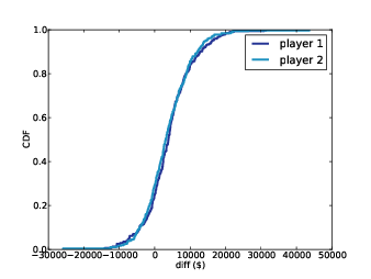
Figure 6.2: Cumulative distribution (CDF) of the difference between the contestant’s bid and the actual price.
The PDFs in Figure 6.1 estimate the distribution of possible prices. If you were a contestant on the show, you could use this distribution to quantify your prior belief about the price of each showcase (before you see the prizes).
To update these priors, we have to answer these questions:
- What data should we consider and how should we quantify it?
- Can we compute a likelihood function; that is, for each hypothetical value of price, can we compute the conditional likelihood of the data?
To answer these questions, I am going to model the contestant as a price-guessing instrument with known error characteristics. In other words, when the contestant sees the prizes, he or she guesses the price of each prize—ideally without taking into consideration the fact that the prize is part of a showcase—and adds up the prices. Let’s call this total guess.
Under this model, the question we have to answer is, “If the actual price is price, what is the likelihood that the contestant’s estimate would be guess?”
Or if we define
error = price - guess
then we could ask, “What is the likelihood that the contestant’s estimate is off by error?”
To answer this question, we can use the historical data again. Figure 6.2 shows the cumulative distribution of diff, the difference between the contestant’s bid and the actual price of the showcase.
The definition of diff is
diff = price - bid
When diff is negative, the bid is too high. As an aside, we can use this distribution to compute the probability that the contestants overbid: the first contestant overbids 25% of the time; the second contestant overbids 29% of the time.
We can also see that the bids are biased; that is, they are more likely to be too low than too high. And that makes sense, given the rules of the game.
Finally, we can use this distribution to estimate the reliability of the contestants’ guesses. This step is a little tricky because we don’t actually know the contestant’s guesses; we only know what they bid.
So we’ll have to make some assumptions. Specifically, I assume that the distribution of error is Gaussian with mean 0 and the same variance as diff.
The Player class implements this model:
class Player(object):

    def __init__(self, prices, bids, diffs):
        self.pdf_price = thinkbayes.EstimatedPdf(prices)
        self.cdf_diff = thinkbayes.MakeCdfFromList(diffs)

        mu = 0
        sigma = numpy.std(diffs)
        self.pdf_error = thinkbayes.GaussianPdf(mu, sigma)
prices is a sequence of showcase prices, bids is a sequence of bids, and diffs is a sequence of diffs, where again diff = price - bid.
pdf_price is the smoothed PDF of prices, estimated by KDE.
cdf_diff is the cumulative distribution of diff,
which we saw in Figure 6.2. And pdf_error
is the PDF that characterizes the distribution of errors; where
error = price - guess.
Again, we use the variance of diff to estimate the variance of error. This estimate is not perfect because contestants’ bids are sometimes strategic; for example, if Player 2 thinks that Player 1 has overbid, Player 2 might make a very low bid. In that case diff does not reflect error. If this happens a lot, the observed variance in diff might overestimate the variance in error. Nevertheless, I think it is a reasonable modeling decision.
As an alternative, someone preparing to appear on the show could estimate their own distribution of error by watching previous shows and recording their guesses and the actual prices.
6.6 Likelihood
Now we are ready to write the likelihood function. As usual, I define a new class that extends thinkbayes.Suite:
class Price(thinkbayes.Suite):

    def __init__(self, pmf, player):
        thinkbayes.Suite.__init__(self, pmf)
        self.player = player
pmf represents the prior distribution and player is a Player object as described in the previous section. Here’s Likelihood:
    def Likelihood(self, data, hypo):
        price = hypo
        guess = data

        error = price - guess
        like = self.player.ErrorDensity(error)

        return like
hypo is the hypothetical price of the showcase. data is the contestant’s best guess at the price. error is the difference, and like is the likelihood of the data, given the hypothesis.
ErrorDensity is defined in Player:
# class Player:

    def ErrorDensity(self, error):
        return self.pdf_error.Density(error)
ErrorDensity works by evaluating pdf_error at
the given value of error.
The result is a probability density, so it is not really a probability.
But remember that Likelihood doesn’t
need to compute a probability; it only has to compute something proportional to a probability. As long as the constant of
proportionality is the same for all likelihoods, it gets canceled out
when we normalize the posterior distribution.
And therefore, a probability density is a perfectly good likelihood.
6.7 Update
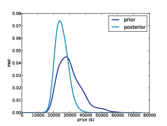
Figure 6.3: Prior and posterior distributions for Player 1, based on a best guess of $20,000.
Player provides a method that takes the contestant’s guess and computes the posterior distribution:
# class Player

    def MakeBeliefs(self, guess):
        pmf = self.PmfPrice()
        self.prior = Price(pmf, self)
        self.posterior = self.prior.Copy()
        self.posterior.Update(guess)
PmfPrice generates a discrete approximation to the PDF of price, which we use to construct the prior.
PmfPrice uses MakePmf, which
evaluates pdf_price at a sequence of values:
# class Player

    n = 101
    price_xs = numpy.linspace(0, 75000, n)

    def PmfPrice(self):
        return self.pdf_price.MakePmf(self.price_xs)
To construct the posterior, we make a copy of the prior and then invoke Update, which invokes Likelihood for each hypothesis, multiplies the priors by the likelihoods, and renormalizes.
So let’s get back to the original scenario. Suppose you are Player 1 and when you see your showcase, your best guess is that the total price of the prizes is $20,000.
Figure 6.3 shows prior and posterior beliefs about the actual price. The posterior is shifted to the left because your guess is on the low end of the prior range.
On one level, this result makes sense. The most likely value in the prior is $27,750, your best guess is $20,000, and the mean of the posterior is somewhere in between: $25,096.
On another level, you might find this result bizarre, because it suggests that if you think the price is $20,000, then you should believe the price is $24,000.
To resolve this apparent paradox, remember that you are combining two sources of information, historical data about past showcases and guesses about the prizes you see.
We are treating the historical data as the prior and updating it based on your guesses, but we could equivalently use your guess as a prior and update it based on historical data.
If you think of it that way, maybe it is less surprising that the most likely value in the posterior is not your original guess.
6.8 Optimal bidding
Now that we have a posterior distribution, we can use it to compute the optimal bid, which I define as the bid that maximizes expected return (see http://en.wikipedia.org/wiki/Expected_return).
I’m going to present the methods in this section top-down, which means I will show you how they are used before I show you how they work. If you see an unfamiliar method, don’t worry; the definition will be along shortly.
To compute optimal bids, I wrote a class called GainCalculator:
class GainCalculator(object):

    def __init__(self, player, opponent):
        self.player = player
        self.opponent = opponent
player and opponent are Player objects.
GainCalculator provides ExpectedGains, which computes a sequence of bids and the expected gain for each bid:
    def ExpectedGains(self, low=0, high=75000, n=101):
        bids = numpy.linspace(low, high, n)

        gains = [self.ExpectedGain(bid) for bid in bids]

        return bids, gains
low and high specify the range of possible bids; n is the number of bids to try.
ExpectedGains calls ExpectedGain, which computes expected gain for a given bid:
    def ExpectedGain(self, bid):
        suite = self.player.posterior
        total = 0
        for price, prob in sorted(suite.Items()):
            gain = self.Gain(bid, price)
            total += prob * gain
        return total
ExpectedGain loops through the values in the posterior and computes the gain for each bid, given the actual prices of the showcase. It weights each gain with the corresponding probability and returns the total.
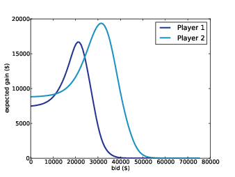
Figure 6.4: Expected gain versus bid in a scenario where Player 1’s best guess is $20,000 and Player 2’s best guess is $40,000.
ExpectedGain invokes Gain, which takes a bid and an actual price and returns the expected gain:
    def Gain(self, bid, price):
        if bid > price:
            return 0

        diff = price - bid
        prob = self.ProbWin(diff)

        if diff <= 250:
            return 2 * price * prob
        else:
            return price * prob
If you overbid, you get nothing. Otherwise we compute the difference between your bid and the price, which determines your probability of winning.
If diff is less than $250, you win both showcases. For simplicity, I assume that both showcases have the same price. Since this outcome is rare, it doesn’t make much difference.
Finally, we have to compute the probability of winning based on diff:
    def ProbWin(self, diff):
        prob = (self.opponent.ProbOverbid() +
                self.opponent.ProbWorseThan(diff))
        return prob
If your opponent overbids, you win. Otherwise, you have to hope that your opponent is off by more than diff. Player provides methods to compute both probabilities:
# class Player:

    def ProbOverbid(self):
        return self.cdf_diff.Prob(-1)

    def ProbWorseThan(self, diff):
        return 1 - self.cdf_diff.Prob(diff)
This code might be confusing because the computation is now from the point of view of the opponent, who is computing, “What is the probability that I overbid?” and “What is the probability that my bid is off by more than diff?”
Both answers are based on the CDF of diff. If the opponent’s diff is less than or equal to -1, you win. If the opponent’s diff is worse than yours, you win. Otherwise you lose.
Finally, here’s the code that computes optimal bids:
# class Player:

    def OptimalBid(self, guess, opponent):
        self.MakeBeliefs(guess)
        calc = GainCalculator(self, opponent)
        bids, gains = calc.ExpectedGains()
        gain, bid = max(zip(gains, bids))
        return bid, gain
Given a guess and an opponent, OptimalBid computes the posterior distribution, instantiates a GainCalculator, computes expected gains for a range of bids and returns the optimal bid and expected gain. Whew!
Figure 6.4 shows the results for both players, based on a scenario where Player 1’s best guess is $20,000 and Player 2’s best guess is $40,000.
For Player 1 the optimal bid is $21,000, yielding an expected return of almost $16,700. This is a case (which turns out to be unusual) where the optimal bid is actually higher than the contestant’s best guess.
For Player 2 the optimal bid is $31,500, yielding an expected return of almost $19,400. This is the more typical case where the optimal bid is less than the best guess.
6.9 Discussion
One of the features of Bayesian estimation is that the result comes in the form of a posterior distribution. Classical estimation usually generates a single point estimate or a confidence interval, which is sufficient if estimation is the last step in the process, but if you want to use an estimate as an input to a subsequent analysis, point estimates and intervals are often not much help.
In this example, we use the posterior distribution to compute an optimal bid. The return on a given bid is asymmetric and discontinuous (if you overbid, you lose), so it would be hard to solve this problem analytically. But it is relatively simple to do computationally.
Newcomers to Bayesian thinking are often tempted to summarize the posterior distribution by computing the mean or the maximum likelihood estimate. These summaries can be useful, but if that’s all you need, then you probably don’t need Bayesian methods in the first place.
Bayesian methods are most useful when you can carry the posterior distribution into the next step of the analysis to perform some kind of decision analysis, as we did in this chapter, or some kind of prediction, as we see in the next chapter.


