Chapter 7 Caching

7.1 How programs run

In order to understand caching, you have to understand how computers execute programs. For a deep understanding of this topic, you should study computer architecture. My goal in this chapter is to provide a simple model of program execution.

When a program starts, the code (or text) is usually on a hard disk or solid state drive. The operating system creates a new process to run the program, then the “loader” copies the text from storage into main memory and starts the program by calling main.

While the program is running, most of its data is stored in main memory, but some of the data is in registers, which are small units of memory on the CPU. These registers include:

The program counter, or PC, which contains the address (in memory) of the next instruction in the program.
The instruction register, or IR, which contains the machine code instruction currently executing.
The stack pointer, or SP, which contains the address of the stack frame for the current function, which contains its parameters and local variables.
General-purpose registers that hold the data the program is currently working with.
A status register, or flag register, that contains information about the current computation. For example, the flag register usually contains a bit that is set if the result of the previous operation was zero.

When a program is running, the CPU executes the following steps, called the “instruction cycle”:

Fetch: The next instruction is fetched from memory and stored in the instruction register.
Decode: Part of the CPU, called the “control unit”, decodes the instruction and sends signals to the other parts of the CPU.
Execute: Signals from the control unit cause the appropriate computation to occur.

Most computers can execute a few hundred different instructions, called the “instruction set”. But most instructions fall into a few general categories:

Load: Transfers a value from memory to a register.
Arithmetic/logic: Loads operands from registers, performs a mathematical operation, and stores the result in a register.
Store: Transfers a value from a register to memory.
Jump/branch: Changes the program counter, causing the flow of execution to jump to another location in the program. Branches are usually conditional, which means that they check a flag in the flag register and jump only if it is set.

Some instructions sets, including the ubiquitous x86, provide instructions that combine a load and an arithmetic operation.

During each instruction cycle, one instruction is read from the program text. In addition, about half of the instructions in a typical program load or store data. And therein lies one of the fundamental problems of computer architecture: the “memory bottleneck”.

In current computers, a typical core is capable of executing an instruction in less than 1 ns. But the time it takes to transfer data to and from memory is about 100 ns. If the CPU has to wait 100 ns to fetch the next instruction, and another 100 ns to load data, it would complete instructions 200 times slower than what’s theoretically possible. For many computations, memory is the speed limiting factor, not the CPU.

7.2 Cache performance

The solution to this problem, or at least a partial solution, is caching. A “cache” is a small, fast memory that is physically close to the CPU, usually on the same chip.

Actually, current computers typically have several levels of cache: the Level 1 cache, which is the smallest and fastest, might be 1–2 MiB with a access times near 1 ns; the Level 2 cache might have access times near 4 ns, and the Level 3 might take 16 ns.

When the CPU loads a value from memory, it stores a copy in the cache. If the same value is loaded again, the CPU gets the cached copy and doesn’t have to wait for memory.

Eventually the cache gets full. Then, in order to bring something new in, we have to kick something out. So if the CPU loads a value and then loads it again much later, it might not be in cache any more.

The performance of many programs is limited by the effectiveness of the cache. If the instructions and data needed by the CPU are usually in cache, the program can run close to the full speed of the CPU. If the CPU frequently needs data that are not in cache, the program is limited by the speed of memory.

The cache “hit rate”, h, is the fraction of memory accesses that find data in cache; the “miss rate”, m, is the fraction of memory accesses that have to go to memory. If the time to process a cache hit is T_h and the time for a cache miss is T_m, the average time for each memory access is

h T_h + m T_m

Equivalently, we could define the “miss penalty” as the extra time to process a cache miss, T_p = T_m − T_h. Then the average access time is

T_h + m T_p

When the miss rate is low, the average access time can be close to T_h. That is, the program can perform as if memory ran at cache speeds.

7.3 Locality

When a program reads a byte for the first time, the cache usually loads a “block” or “line” of data that includes the requested byte and some of its neighbors. If the program goes on to read one of the neighbors, it will already be in cache.

As an example, suppose the block size is 64 B; you read a string with length 64, and the first byte of the string happens to fall at the beginning of a block. When you load the first byte, you incur a miss penalty, but after that the rest of the string will be in cache. After reading the whole string, the hit rate will be 63/64, about 98%. If the string spans two blocks, you would incur 2 miss penalties. But even then the hit rate would be 62/64, or almost 97%. If you then read the same string again, the hit rate would be 100%.

On the other hand, if the program jumps around unpredictably, reading data from scattered locations in memory, and seldom accessing the same location twice, cache performance would be poor.

The tendency of a program to use the same data more than once is called “temporal locality”. The tendency to use data in nearby locations is called “spatial locality”. Fortunately, many programs naturally display both kinds of locality:

Most programs contain blocks of code with no jumps or branches. Within these blocks, instructions run sequentially, so the access pattern has spatial locality.
In a loop, programs execute the same instructions many times, so the access pattern has temporal locality.
The result of one instruction is often used immediately as an operand of the next instruction, so the data access pattern has temporal locality.
When a program executes a function, its parameters and local variables are stored together on the stack; accessing these values has spatial locality.
One of the most common processing patterns is to read or write the elements of an array sequentially; this pattern also has spatial locality.

The next section explores the relationship between a program’s access pattern and cache performance.

7.4 Measuring cache performance

When I was a graduate student at U.C. Berkeley I was a teaching assistant for Computer Architecture with Brian Harvey. One of my favorite exercises involved a program that iterates through an array and measures the average time to read and write an element. By varying the size of the array, it is possible to infer the size of the cache, the block size, and some other attributes.

My modified version of this program is in the cache directory of the repository for this book (see Section 0.1).

The important part of the program is this loop:

    iters = 0;
    do {
        sec0 = get_seconds();

        for (index = 0; index < limit; index += stride) 
            array[index] = array[index] + 1;
        
        iters = iters + 1; 
        sec = sec + (get_seconds() - sec0);
        
    } while (sec < 0.1);

The inner for loop traverses the array. limit determines how much of the array it traverses; stride determines how many elements it skips over. For example, if limit is 16 and stride is 4, the loop would access elements 0, 4, 8, and 12.

sec keeps track of the total CPU time used by the inner loop. The outer loop runs until sec exceeds 0.1 seconds, which is long enough that we can compute the average time with sufficient precision.

get_seconds uses the system call clock_gettime, converts to seconds, and returns the result as a double:

double get_seconds(){
    struct timespec ts;
    clock_gettime(CLOCK_PROCESS_CPUTIME_ID, &ts);
    return ts.tv_sec + ts.tv_nsec / 1e9;
}

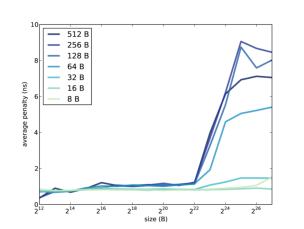
Figure 7.1: Average miss penalty as a function of array size and stride.

To isolate the time to access the elements of the array, the program runs a second loop that is almost identical except that the inner loop doesn’t touch the array; it always increments the same variable:

    iters2 = 0;
    do {
        sec0 = get_seconds();
        
        for (index = 0; index < limit; index += stride) 
            temp = temp + index;
        
        iters2 = iters2 + 1;
        sec = sec - (get_seconds() - sec0);

    } while (iters2 < iters);

The second loop runs the same number of iterations as the first. After each iteration, it subtracts the elapsed time from sec. When the loop completes, sec contains the total time for all array accesses, minus the total time it took to increment temp. This difference is the total miss penalty incurred by all accesses. Finally, we divide by the number of accesses to get the average miss penalty per access, in ns:

sec * 1e9 / iters / limit * stride

If you compile and run cache.c you should see output like this:

Size:    4096 Stride:       8 read+write: 0.8633 ns
Size:    4096 Stride:      16 read+write: 0.7023 ns
Size:    4096 Stride:      32 read+write: 0.7105 ns
Size:    4096 Stride:      64 read+write: 0.7058 ns

If you have Python and matplotlib installed, you can use graph_data.py to graph the results. Figure 7.1 shows the results when I ran it on a Dell Optiplex 7010. Notice that the array size and stride are reported in bytes, not number of array elements.

Take a minute to consider this graph, and see what you can infer about the cache. Here are some things to think about:

The program reads through the array many times, so it has plenty of temporal locality. If the entire array fits in cache, we expect the average miss penalty to be near 0.
When the stride is 4 bytes, we read every element of the array, so the program has plenty of spatial locality. If the block size is big enough to contain 64 elements, for example, the hit rate would be 63/64, even if the array does not fit in cache.
If the stride is equal to the block size (or greater), the spatial locality is effectively zero, because each time we read a block, we only access one element. In that case we expect to see the maximum miss penalty.

In summary, we expect good cache performance if the array is smaller than the cache size or if the stride is smaller than the block size. Performance only degrades if the array is bigger than the cache and the stride is large.

In Figure 7.1, cache performance is good, for all strides, as long as the array is less than 2²² B. We can infer that the cache size is near 4 MiB; in fact, according to the specs, it is 3 MiB.

When the stride is 8, 16, or 32 B, cache performance is good. At 64 B it starts to degrade, and for larger strides the average miss penalty is about 9 ns. We can infer that the block size near 128 B.

Many processors use “multi-level caches” that include a small, fast cache and a bigger, slower cache. In this example, it looks like the miss penalty increases a little when the array size is bigger than 2¹⁴ B, so it’s possible that this processor also has a 16 KB cache with an access time less than 1 ns.

7.5 Programming for cache performance

Memory caching is implemented in hardware, so most of the time programmers don’t need to know much about it. But if you know how caches work, you can write programs that use them more effectively.

For example, if you are working with a large array, it might be faster to traverse the array once, performing several operations with each element, rather than traversing the array several times.

If you are working with a 2-D array, it might be stored as an array of rows. If you traverse through the elements, it would be faster to go row-wise, with stride equal to the element size, rather than column-wise, with stride equal to the row length.

Linked data structures don’t always exhibit spatial locality, because the nodes aren’t necessarily contiguous in memory. But if you allocate many nodes at the same time, they are usually co-located in the heap. Or, even better, if you allocate an array of nodes all at once, you know they will be contiguous.

Recursive strategies like mergesort often have good cache behavior because they break big arrays into smaller pieces and then work with the pieces. Sometimes these algorithms can be tuned to take advantage of cache behavior.

For applications where performance is critical, it is possible to design algorithms tailored to the size of the cache, the block size, and other hardware characterstics. Algorithms like that are called “cache-aware”. The obvious drawback of cache-aware algorithms is that they are hardware-specific.

7.6 The memory hierarchy

At some point during this chapter, a question like the following might have occurred to you: “If caches are so much faster than main memory, why not make a really big cache and forget about memory?”

Without going too far into computer architecture, there are two reasons: electronics and economics. Caches are fast because they are small and close to the CPU, which minimizes delays due to capacitance and signal propagation. If you make a cache big, it will be slower.

Also, caches take up space on the processor chip, and bigger chips are more expensive. Main memory is usually dynamic random-access memory (DRAM), which uses only one transistor and one capacitor per bit, so it is possible to pack more memory into the same amount of space. But this way of implementing memory is slower than the way caches are implemented.

Also main memory is usually packaged in a dual in-line memory module (DIMM) that includes 16 or more chips. Several small chips are cheaper than one big one.

The trade-off between speed, size, and cost is the fundamental reason for caching. If there were one memory technology that was fast, big, and cheap, we wouldn’t need anything else.

The same principle applies to storage as well as memory. Solid state drives (SSD) are fast, but they are more expensive than hard drives (HDD), so they tend to be smaller. Tape drives are even slower than hard drives, but they can store large amounts of data relatively cheaply.

The following table shows typical access times, sizes, and costs for each of these technologies.

Device	Access	Typical	Cost
	time	size
Register	0.5 ns	256 B	?
Cache	1 ns	2 MiB	?
DRAM	100 ns	4 GiB	$10 / GiB
SSD	10 µs	100 GiB	$1 / GiB
HDD	5 ms	500 GiB	$0.25 / GiB
Tape	minutes	1–2 TiB	$0.02 / GiB

The number and size of registers depends on details of the architecture. Current computers have about 32 general-purpose registers, each storing one “word”. On a 32-bit computer, a word is 32 bits or 4 B. On a 64-bit computer, a word is 64 bits or 8 B. So the total size of the register file is 100–300 B.

The cost of registers and caches is hard to quantify. They contribute to the cost of the chips they are on, but consumers don’t see that cost directly.

For the other numbers in the table, I looked at the specifications for typical hardware for sale from online computer hardware stores. By the time you read this, these numbers will be obsolete, but they give you an idea of what the performance and cost gaps looked like at one point in time.

These technologies make up the “memory hierarchy” (note that this use of “memory” also includes storage). Each level of the hierarchy is bigger and slower than the one above it. And in some sense, each level acts as a cache for the one below it. You can think of main memory as a cache for programs and data that are stored permanently on SSDs and HHDs. And if you are working with very large datasets stored on tape, you could use hard drives to cache one subset of the data at a time.

7.7 Caching policy

The memory hierarchy suggests a framework for thinking about caching. At every level of the hierarchy, we have to address four fundamental questions of caching:

Who moves data up and down the hierarchy? At the top of the hierarchy, register allocation is usually done by the compiler. Hardware on the CPU handles the memory cache. Users implicitly move data from storage to memory when they execute programs and open files. But the operating system also moves data back and forth between memory and storage. At the bottom of the hierarchy, administrators move data explicitly between disk and tape.
What gets moved? In general, block sizes are small at the top of the hierarchy and bigger at the bottom. In a memory cache, a typical block size is 128 B. Pages in memory might be 4 KiB, but when the operating system reads a file from disk, it might read 10s or 100s of blocks at a time.
When does data get moved? In the most basic cache, data gets moved into cache when it is used for the first time. But many caches use some kind of “prefetching”, meaning that data is loaded before it is explicitly requested. We have already seen one form of prefetching: loading an entire block when only part of it is requested.
Where in the cache does the data go? When the cache is full, we can’t bring anything in without kicking something out. Ideally, we want to keep data that will be used again soon and replace data that won’t.

The answers to these questions make up the “cache policy”. Near the top of the hierarchy, cache policies tend to be simple because they have to be fast and they are implemented in hardware. Near the bottom of the hierarchy, there is more time to make decisions, and well-designed policies can make a big difference.

Most cache policies are based on the principle that history repeats itself; if we have information about the recent past, we can use it to predict the immediate future. For example, if a block of data has been used recently, we expect it to be used again soon. This principle suggests a replacement policy called “least recently used,” or LRU, which removes from the cache a block of data that has not been used recently. For more on this topic, see http://en.wikipedia.org/wiki/Cache_algorithms.

7.8 Paging

In systems with virtual memory, the operating system can move pages back and forth between memory and storage. As I mentioned in Section 6.2, this mechanism is called “paging” or sometimes “swapping”.

Here’s how the process works:

Suppose Process A calls malloc to allocate a chunk. If there is no free space in the heap with the requested size, malloc calls sbrk to ask the operating system for more memory.
If there is a free page in physical memory, the operating system adds it to the page table for Process A, creating a new range of valid virtual addresses.
If there are no free pages, the paging system chooses a “victim page” belonging to Process B. It copies the contents of the victim page from memory to disk, then it modifies the page table for Process B to indicate that this page is “swapped out”.
Once the data from Process B is written, the page can be reallocated to Process A. To prevent Process A from reading Process B’s data, the page should be cleared.
At this point the call to sbrk can return, giving malloc additional space in the heap. Then malloc allocates the requested chunk and returns. Process A can resume.
When Process A completes, or is interrupted, the scheduler might allow Process B to resume. When Process B accesses a page that has been swapped out, the memory management unit notices that the page is “invalid” and causes an interrupt.
When the operating system handles the interrupt, it sees that the page is swapped out, so it transfers the page back from disk to memory.
Once the page is swapped in, Process B can resume.

When paging works well, it can greatly improve the utilization of physical memory, allowing more processes to run in less space. Here’s why:

Most processes don’t use all of their allocated memory. Many parts of the text segment are never executed, or execute once and never again. Those pages can be swapped out without causing any problems.
If a program leaks memory, it might leave allocated space behind and never access it again. By swapping those pages out, the operating system can effectively plug the leak.
On most systems, there are processes like daemons that sit idle most of the time and only occasionally “wake up” to respond to events. While they are idle, these processes can be swapped out.
A user might have many windows open, but only a few are active at a time. The inactive processes can be swapped out.
Also, there might be many processes running the same program. These processes can share the same text and static segments, avoiding the need to keep multiple copies in physical memory.

If you add up the total memory allocated to all processes, it can greatly exceed the size of physical memory, and yet the system can still behave well.

Up to a point.

When a process accesses a page that’s swapped out, it has to get the data back from disk, which can take several milliseconds. The delay is often noticeable. If you leave a window idle for a long time and then switch back to it, it might start slowly, and you might hear the disk drive working while pages are swapped in.

Occasional delays like that might be acceptable, but if you have too many processes using too much space, they start to interfere with each other. When Process A runs, it evicts the pages Process B needs. Then when B runs, it evicts the pages A needs. When this happens, both processes slow to a crawl and the system can become unresponsive. This scenario is called “thrashing”.

In theory, operating systems could avoid thrashing by detecting an increase in paging and blocking or killing processes until the system is responsive again. But as far as I can tell, most systems don’t do this, or don’t do it well; it is often left to users to limit their use of physical memory or try to recover when thrashing occurs.