|
This HTML version of is provided for convenience, but it is not the best format for the book. In particular, some of the symbols are not rendered correctly. You might prefer to read the PDF version, or you can buy a hardcopy here. Chapter 3 Cumulative distribution functions3.1 The class size paradoxAt many American colleges and universities, the student-to-faculty ratio is about 10:1. But students are often surprised to discover that their average class size is bigger than 10. There are two reasons for the discrepancy:
The first effect is obvious (at least once it is pointed out); the second is more subtle. So let’s look at an example. Suppose that a college offers 65 classes in a given semester, with the following distribution of sizes: size count 5- 9 8 10-14 8 15-19 14 20-24 4 25-29 6 30-34 12 35-39 8 40-44 3 45-49 2 If you ask the Dean for the average class size, he would construct a PMF, compute the mean, and report that the average class size is 24. But if you survey a group of students, ask them how many students are in their classes, and compute the mean, you would think that the average class size was higher. Exercise 1
Build a PMF of these data and compute the mean as perceived by the
Dean. Since the data have been grouped in bins, you can use the
mid-point of each bin.
Now find the distribution of class sizes as perceived by students and compute its mean. Suppose you want to find the distribution of class sizes at a college, but you can’t get reliable data from the Dean. An alternative is to choose a random sample of students and ask them the number of students in each of their classes. Then you could compute the PMF of their responses. The result would be biased because large classes would be oversampled, but you could estimate the actual distribution of class sizes by applying an appropriate transformation to the observed distribution. Write a function called You can download a solution to this problem from http://thinkstats.com/class_size.py. Exercise 2
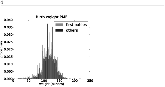
In most foot races, everyone starts at the same time. If you are a fast runner, you usually pass a lot of people at the beginning of the race, but after a few miles everyone around you is going at the same speed. When I ran a long-distance (209 miles) relay race for the first time, I noticed an odd phenomenon: when I overtook another runner, I was usually much faster, and when another runner overtook me, he was usually much faster. At first I thought that the distribution of speeds might be bimodal; that is, there were many slow runners and many fast runners, but few at my speed. Then I realized that I was the victim of selection bias. The race was unusual in two ways: it used a staggered start, so teams started at different times; also, many teams included runners at different levels of ability. As a result, runners were spread out along the course with little relationship between speed and location. When I started running my leg, the runners near me were (pretty much) a random sample of the runners in the race. So where does the bias come from? During my time on the course, the chance of overtaking a runner, or being overtaken, is proportional to the difference in our speeds. To see why, think about the extremes. If another runner is going at the same speed as me, neither of us will overtake the other. If someone is going so fast that they cover the entire course while I am running, they are certain to overtake me. Write a function called BiasPmf that takes a Pmf representing the actual distribution of runners’ speeds, and the speed of a running observer, and returns a new Pmf representing the distribution of runners’ speeds as seen by the observer. To test your function, get the distribution of speeds from a normal road race (not a relay). I wrote a program that reads the results from the James Joyce Ramble 10K in Dedham MA and converts the pace of each runner to MPH. Download it from http://thinkstats.com/relay.py. Run it and look at the PMF of speeds. Now compute the distribution of speeds you would observe if you ran a relay race at 7.5 MPH with this group of runners. You can download a solution from http://thinkstats.com/relay_soln.py 3.2 The limits of PMFsPMFs work well if the number of values is small. But as the number of values increases, the probability associated with each value gets smaller and the effect of random noise increases. For example, we might be interested in the distribution of birth
weights. In the NSFG data, the variable
Overall, these distributions resemble the familiar “bell curve,” with many values near the mean and a few values much higher and lower. But parts of this figure are hard to interpret. There are many spikes and valleys, and some apparent differences between the distributions. It is hard to tell which of these features are significant. Also, it is hard to see overall patterns; for example, which distribution do you think has the higher mean? These problems can be mitigated by binning the data; that is, dividing the domain into non-overlapping intervals and counting the number of values in each bin. Binning can be useful, but it is tricky to get the size of the bins right. If they are big enough to smooth out noise, they might also smooth out useful information. An alternative that avoids these problems is the cumulative distribution function, or CDF. But before we can get to that, we have to talk about percentiles. 3.3 PercentilesIf you have taken a standardized test, you probably got your results in the form of a raw score and a percentile rank. In this context, the percentile rank is the fraction of people who scored lower than you (or the same). So if you are “in the 90th percentile,” you did as well as or better than 90% of the people who took the exam. Here’s how you could compute the percentile rank of a value,
def PercentileRank(scores, your_score):
    count = 0
    for score in scores:
        if score <= your_score:
            count += 1

    percentile_rank = 100.0 * count / len(scores)
    return percentile_rank
For example, if the scores in the sequence were 55, 66, 77, 88 and 99, and you got the 88, then your percentile rank would be 100 * 4 / 5 which is 80. If you are given a value, it is easy to find its percentile rank; going the other way is slightly harder. If you are given a percentile rank and you want to find the corresponding value, one option is to sort the values and search for the one you want: def Percentile(scores, percentile_rank):
scores.sort()
for score in scores:
if PercentileRank(scores, score) >= percentile_rank:
return score
The result of this calculation is a percentile. For example, the 50th percentile is the value with percentile rank 50. In the distribution of exam scores, the 50th percentile is 77. Exercise 3
This implementation of Percentile is not very efficient. A
better approach is to use the percentile rank to compute the index of
the corresponding percentile. Write a version of Percentile that
uses this algorithm. You can download a solution from http://thinkstats.com/score_example.py. Exercise 4
Optional: If you only want to compute one percentile, it is not
efficient to sort the scores. A better option is the selection
algorithm, which you can read about at
http://wikipedia.org/wiki/Selection_algorithm.
Write (or find) an implementation of the selection algorithm and use it to write an efficient version of Percentile. 3.4 Cumulative distribution functionsNow that we understand percentiles, we are ready to tackle the cumulative distribution function (CDF). The CDF is the function that maps values to their percentile rank in a distribution. The CDF is a function of x, where x is any value that might appear in the distribution. To evaluate CDF(x) for a particular value of x, we compute the fraction of the values in the sample less than (or equal to) x. Here’s what that looks like as a function that takes a sample, t, and a value, x: def Cdf(t, x):
count = 0.0
for value in t:
if value <= x:
count += 1.0
prob = count / len(t)
return prob
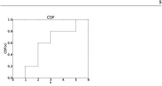
This function should look familiar; it is almost identical to PercentileRank, except that the result is in a probability in the range 0–1 rather than a percentile rank in the range 0–100. As an example, suppose a sample has the values {1, 2, 2, 3, 5}. Here are some values from its CDF: CDF(0) = 0 CDF(1) = 0.2 CDF(2) = 0.6 CDF(3) = 0.8 CDF(4) = 0.8 CDF(5) = 1 We can evaluate the CDF for any value of x, not just values that appear in the sample. If x is less than the smallest value in the sample, CDF(x) is 0. If x is greater than the largest value, CDF(x) is 1.
Figure 3.2 is a graphical representation of this CDF. The CDF of a sample is a step function. In the next chapter we will see distributions whose CDFs are continuous functions. 3.5 Representing CDFsI have written a module called Cdf that provides a class named Cdf that represents CDFs. You can read the documentation of this module at http://thinkstats.com/Cdf.html and you can download it from http://thinkstats.com/Cdf.py. Cdfs are implemented with two sorted lists: xs, which contains the values, and ps, which contains the probabilities. The most important methods Cdfs provide are:
Because xs and ps are sorted, these operations can use the bisection algorithm, which is efficient. The run time is proportional to the logarithm of the number of values; see http://wikipedia.org/wiki/Time_complexity. Cdfs also provide Render, which returns two lists, xs and ps, suitable for plotting the CDF. Because the CDF is a step function, these lists have two elements for each unique value in the distribution. The Cdf module provides several functions for making Cdfs, including MakeCdfFromList, which takes a sequence of values and returns their Cdf. Finally, myplot.py provides functions named Cdf and Cdfs that plot Cdfs as lines. Exercise 5
Download Cdf.py and relay.py (see
Exercise 2) and generate a plot that shows the CDF of
running speeds. Which gives you a better sense of the shape of the
distribution, the PMF or the CDF? You can download a solution
from http://thinkstats.com/relay_cdf.py.
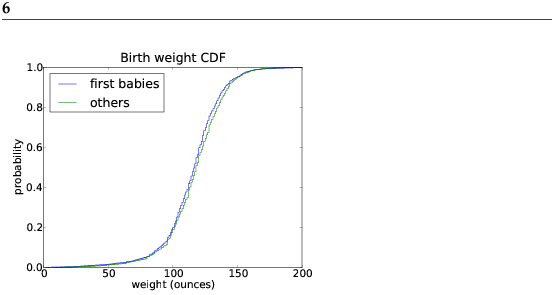
3.6 Back to the survey dataFigure 3.3 shows the CDFs of birth weight for first babies and others in the NSFG dataset.
This figure makes the shape of the distributions, and the differences between them, much clearer. We can see that first babies are slightly lighter throughout the distribution, with a larger discrepancy above the mean. Exercise 6
How much did you weigh at birth? If you don’t know, call your mother
or someone else who knows. Using the pooled data (all live births),
compute the distribution of birth weights and use it to find your
percentile rank. If you were a first baby, find your percentile rank
in the distribution for first babies. Otherwise use the distribution
for others. If you are in the 90th percentile or higher, call your
mother back and apologize. Exercise 7
Suppose you and your classmates compute the percentile rank of your
birth weights and then compute the CDF of the percentile ranks. What do
you expect it to look like? Hint: what fraction of the class do you
expect to be above the median?
3.7 Conditional distributionsA conditional distribution is the distribution of a subset of the data which is selected according to a condition. For example, if you are above average in weight, but way above average in height, then you might be relatively light for your height. Here’s how you could make that claim more precise.
Percentile ranks are useful for comparing measurements from different tests, or tests applied to different groups. For example, people who compete in foot races are usually grouped by age and gender. To compare people in different groups, you can convert race times to percentile ranks. Exercise 8
I recently ran the James Joyce Ramble 10K
in Dedham MA. The results are available from
http://coolrunning.com/results/10/ma/Apr25_27thAn_set1.shtml.
Go to that page and find my results. I came in 97th in a field
of 1633, so what is my percentile rank in the field?
In my division (M4049 means “male between 40 and 49 years of age”) I came in 26th out of 256. What is my percentile rank in my division? If I am still running in 10 years (and I hope I am), I will be in the M5059 division. Assuming that my percentile rank in my division is the same, how much slower should I expect to be? I maintain a friendly rivalry with a student who is in the F2039 division. How fast does she have to run her next 10K to “beat” me in terms of percentile ranks? 3.8 Random numbersCDFs are useful for generating random numbers with a given distribution. Here’s how:
It might not be obvious why this works, but since it is easier to implement than to explain, let’s try it out. Exercise 9
Write a function called Sample, that takes a Cdf and
an integer, n, and returns a list of n values chosen at
random from the Cdf. Hint: use random.random.
You will find a solution to this exercise in Cdf.py.
Using the distribution of birth weights from the NSFG, generate a random sample with 1000 elements. Compute the CDF of the sample. Make a plot that shows the original CDF and the CDF of the random sample. For large values of n, the distributions should be the same. This process, generating a random sample based on a measured sample, is called resampling. There are two ways to draw a sample from a population: with and without replacement. If you imagine drawing marbles from an urn1, “replacement” means putting the marbles back as you go (and stirring), so the population is the same for every draw. “Without replacement,” means that each marble can only be drawn once, so the remaining population is different after each draw. In Python, sampling with replacement can be implemented with random.random to choose a percentile rank, or random.choice to choose an element from a sequence. Sampling without replacement is provided by random.sample. Exercise 10
The numbers generated by random.random are supposed to be
uniform between 0 and 1; that is, every value in the range
should have the same probability. Generate 1000 numbers from random.random and plot their PMF and CDF. Can you tell whether they are uniform? You can read about the uniform distribution at http://wikipedia.org/wiki/Uniform_distribution_(discrete). 3.9 Summary statistics revisitedOnce you have computed a CDF, it is easy to compute other summary statistics. The median is just the 50th percentile2. The 25th and 75th percentiles are often used to check whether a distribution is symmetric, and their difference, which is called the interquartile range, measures the spread. Exercise 11
Write a function called Median that takes a Cdf and computes the
median, and one called Interquartile that computes
the interquartile range. Compute the 25th, 50th, and 75th percentiles of the birth weight CDF. Do these values suggest that the distribution is symmetric? 3.10 Glossary
|
Like this book?
Are you using one of our books in a class?We'd like to know about it. Please consider filling out this short survey.
|