


This HTML version of
You might prefer to read the PDF version, or you can buy a hard copy from Amazon.
Chapter 3 Estimation
3.1 The dice problem
Suppose I have a box of dice that contains a 4-sided die, a 6-sided die, an 8-sided die, a 12-sided die, and a 20-sided die. If you have ever played Dungeons & Dragons, you know what I am talking about.
Suppose I select a die from the box at random, roll it, and get a 6. What is the probability that I rolled each die?
Let me suggest a three-step strategy for approaching a problem like this.
- Choose a representation for the hypotheses.
- Choose a representation for the data.
- Write the likelihood function.
In previous examples I used strings to represent hypotheses and data, but for the die problem I’ll use numbers. Specifically, I’ll use the integers 4, 6, 8, 12, and 20 to represent hypotheses:
suite = Dice([4, 6, 8, 12, 20])
And integers from 1 to 20 for the data. These representations make it easy to write the likelihood function:
class Dice(Suite):
    def Likelihood(self, data, hypo):
        if hypo < data:
            return 0
        else:
            return 1.0/hypo
Here’s how Likelihood works. If hypo<data, that
means the roll is greater than the number of sides on the die.
That can’t happen, so the likelihood is 0.
Otherwise the question is, “Given that there are hypo
sides, what is the chance of rolling data?” The
answer is 1/hypo, regardless of data.
Here is the statement that does the update (if I roll a 6):
suite.Update(6)
And here is the posterior distribution:
4 0.0
6 0.392156862745
8 0.294117647059
12 0.196078431373
20 0.117647058824
After we roll a 6, the probability for the 4-sided die is 0. The most likely alternative is the 6-sided die, but there is still almost a 12% chance for the 20-sided die.
What if we roll a few more times and get 6, 8, 7, 7, 5, and 4?
    for roll in [6, 8, 7, 7, 5, 4]:
        suite.Update(roll)
With this data the 6-sided die is eliminated, and the 8-sided die seems quite likely. Here are the results:
4 0.0
6 0.0
8 0.943248453672
12 0.0552061280613
20 0.0015454182665
Now the probability is 94% that we are rolling the 8-sided die, and less than 1% for the 20-sided die.
The dice problem is based on an example I saw in Sanjoy Mahajan’s class on Bayesian inference. You can download the code in this section from http://thinkbayes.com/dice.py. For more information see Section 0.3.
3.2 The locomotive problem
I found the locomotive problem in Frederick Mosteller’s, Fifty Challenging Problems in Probability with Solutions (Dover, 1987):
“A railroad numbers its locomotives in order 1..N. One day you see a locomotive with the number 60. Estimate how many locomotives the railroad has.”
Based on this observation, we know the railroad has 60 or more locomotives. But how many more? To apply Bayesian reasoning, we can break this problem into two steps:
- What did we know about N before we saw the data?
- For any given value of N, what is the likelihood of seeing the data (a locomotive with number 60)?
The answer to the first question is the prior. The answer to the second is the likelihood.
Figure 3.1: Posterior distribution for the locomotive problem, based on a uniform prior.

We don’t have much basis to choose a prior, but we can start with something simple and then consider alternatives. Let’s assume that N is equally likely to be any value from 1 to 1000.
hypos = xrange(1, 1001)
Now all we need is a likelihood function. In a hypothetical fleet of N locomotives, what is the probability that we would see number 60? If we assume that there is only one train-operating company (or only one we care about) and that we are equally likely to see any of its locomotives, then the chance of seeing any particular locomotive is 1/N.
Here’s the likelihood function:
class Train(Suite):
    def Likelihood(self, data, hypo):
        if hypo < data:
            return 0
        else:
            return 1.0/hypo
This might look familiar; the likelihood functions for the locomotive problem and the dice problem are identical.
Here’s the update:
    suite = Train(hypos)
    suite.Update(60)
There are too many hypotheses to print, so I plotted the results in Figure 3.1. Not surprisingly, all values of N below 60 have been eliminated.
The most likely value, if you had to guess, is 60. That might not seem like a very good guess; after all, what are the chances that you just happened to see the train with the highest number? Nevertheless, if you want to maximize the chance of getting the answer exactly right, you should guess 60.
But maybe that’s not the right goal. An alternative is to compute the mean of the posterior distribution:
def Mean(suite):
    total = 0
    for hypo, prob in suite.Items():
        total += hypo * prob
    return total

print Mean(suite)
Or you could use the very similar method provided by Pmf:
print suite.Mean()
The mean of the posterior is 333, so that might be a good guess if you wanted to minimize error. If you played this guessing game over and over, using the mean of the posterior as your estimate would minimize the mean squared error over the long run (see http://en.wikipedia.org/wiki/Minimum_mean_square_error).
You can download this example from http://thinkbayes.com/train.py. For more information see Section 0.3.
3.3 What about that prior?
To make any progress on the locomotive problem we had to make assumptions, and some of them were pretty arbitrary. In particular, we chose a uniform prior from 1 to 1000, without much justification for choosing 1000, or for choosing a uniform distribution.
It is not crazy to believe that a railroad company might operate 1000 locomotives, but a reasonable person might guess more or fewer. So we might wonder whether the posterior distribution is sensitive to these assumptions. With so little data—only one observation—it probably is.
Recall that with a uniform prior from 1 to 1000, the mean of the posterior is 333. With an upper bound of 500, we get a posterior mean of 207, and with an upper bound of 2000, the posterior mean is 552.
So that’s bad. There are two ways to proceed:
- Get more data.
- Get more background information.
With more data, posterior distributions based on different priors tend to converge. For example, suppose that in addition to train 60 we also see trains 30 and 90. We can update the distribution like this:
    for data in [60, 30, 90]:
        suite.Update(data)
With these data, the means of the posteriors are
| Upper | Posterior |
| Bound | Mean |
| 500 | 152 |
| 1000 | 164 |
| 2000 | 171 |
So the differences are smaller.
3.4 An alternative prior
Figure 3.2: Posterior distribution based on a power law prior, compared to a uniform prior.
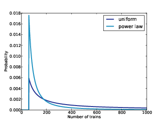
If more data are not available, another option is to improve the priors by gathering more background information. It is probably not reasonable to assume that a train-operating company with 1000 locomotives is just as likely as a company with only 1.
With some effort, we could probably find a list of companies that operate locomotives in the area of observation. Or we could interview an expert in rail shipping to gather information about the typical size of companies.
But even without getting into the specifics of railroad economics, we can make some educated guesses. In most fields, there are many small companies, fewer medium-sized companies, and only one or two very large companies. In fact, the distribution of company sizes tends to follow a power law, as Robert Axtell reports in Science (see http://www.sciencemag.org/content/293/5536/1818.full.pdf).
This law suggests that if there are 1000 companies with fewer than 10 locomotives, there might be 100 companies with 100 locomotives, 10 companies with 1000, and possibly one company with 10,000 locomotives.
Mathematically, a power law means that the number of companies with a given size is inversely proportional to size, or
| PMF(x) ∝ | ⎛ ⎜ ⎜ ⎝ |
| ⎞ ⎟ ⎟ ⎠ |
|
where PMF(x) is the probability mass function of x and α is a parameter that is often near 1.
We can construct a power law prior like this:
class Train(Dice):

    def __init__(self, hypos, alpha=1.0):
        Pmf.__init__(self)
        for hypo in hypos:
            self.Set(hypo, hypo**(-alpha))
        self.Normalize()
And here’s the code that constructs the prior:
    hypos = range(1, 1001)
    suite = Train(hypos)
Again, the upper bound is arbitrary, but with a power law prior, the posterior is less sensitive to this choice.
Figure 3.2 shows the new posterior based on the power law, compared to the posterior based on the uniform prior. Using the background information represented in the power law prior, we can all but eliminate values of N greater than 700.
If we start with this prior and observe trains 30, 60, and 90, the means of the posteriors are
| Upper | Posterior |
| Bound | Mean |
| 500 | 131 |
| 1000 | 133 |
| 2000 | 134 |
Now the differences are much smaller. In fact, with an arbitrarily large upper bound, the mean converges on 134.
So the power law prior is more realistic, because it is based on general information about the size of companies, and it behaves better in practice.
You can download the examples in this section from http://thinkbayes.com/train3.py. For more information see Section 0.3.
3.5 Credible intervals
Once you have computed a posterior distribution, it is often useful to summarize the results with a single point estimate or an interval. For point estimates it is common to use the mean, median, or the value with maximum likelihood.
For intervals we usually report two values computed so that there is a 90% chance that the unknown value falls between them (or any other probability). These values define a credible interval.
A simple way to compute a credible interval is to add up the probabilities in the posterior distribution and record the values that correspond to probabilities 5% and 95%. In other words, the 5th and 95th percentiles.
thinkbayes provides a function that computes percentiles:
def Percentile(pmf, percentage):
    p = percentage / 100.0
    total = 0
    for val, prob in pmf.Items():
        total += prob
        if total >= p:
            return val
And here’s the code that uses it:
    interval = Percentile(suite, 5), Percentile(suite, 95)
    print interval
For the previous example—the locomotive problem with a power law prior and three trains—the 90% credible interval is (91, 243). The width of this range suggests, correctly, that we are still quite uncertain about how many locomotives there are.
3.6 Cumulative distribution functions
In the previous section we computed percentiles by iterating through the values and probabilities in a Pmf. If we need to compute more than a few percentiles, it is more efficient to use a cumulative distribution function, or Cdf.
Cdfs and Pmfs are equivalent in the sense that they contain the same information about the distribution, and you can always convert from one to the other. The advantage of the Cdf is that you can compute percentiles more efficiently.
thinkbayes provides a Cdf class that represents a cumulative distribution function. Pmf provides a method that makes the corresponding Cdf:
cdf = suite.MakeCdf()
And Cdf provides a function named Percentile
interval = cdf.Percentile(5), cdf.Percentile(95)
Converting from a Pmf to a Cdf takes time proportional to the number of values, len(pmf). The Cdf stores the values and probabilities in sorted lists, so looking up a probability to get the corresponding value takes “log time”: that is, time proportional to the logarithm of the number of values. Looking up a value to get the corresponding probability is also logarithmic, so Cdfs are efficient for many calculations.
The examples in this section are in http://thinkbayes.com/train3.py. For more information see Section 0.3.
3.7 The German tank problem
During World War II, the Economic Warfare Division of the American Embassy in London used statistical analysis to estimate German production of tanks and other equipment.1
The Western Allies had captured log books, inventories, and repair records that included chassis and engine serial numbers for individual tanks.
Analysis of these records indicated that serial numbers were allocated by manufacturer and tank type in blocks of 100 numbers, that numbers in each block were used sequentially, and that not all numbers in each block were used. So the problem of estimating German tank production could be reduced, within each block of 100 numbers, to a form of the locomotive problem.
Based on this insight, American and British analysts produced estimates substantially lower than estimates from other forms of intelligence. And after the war, records indicated that they were substantially more accurate.
They performed similar analyses for tires, trucks, rockets, and other equipment, yielding accurate and actionable economic intelligence.
The German tank problem is historically interesting; it is also a nice example of real-world application of statistical estimation. So far many of the examples in this book have been toy problems, but it will not be long before we start solving real problems. I think it is an advantage of Bayesian analysis, especially with the computational approach we are taking, that it provides such a short path from a basic introduction to the research frontier.
3.8 Discussion
Among Bayesians, there are two approaches to choosing prior distributions. Some recommend choosing the prior that best represents background information about the problem; in that case the prior is said to be informative. The problem with using an informative prior is that people might use different background information (or interpret it differently). So informative priors often seem subjective.
The alternative is a so-called uninformative prior, which is intended to be as unrestricted as possible, in order to let the data speak for themselves. In some cases you can identify a unique prior that has some desirable property, like representing minimal prior information about the estimated quantity.
Uninformative priors are appealing because they seem more objective. But I am generally in favor of using informative priors. Why? First, Bayesian analysis is always based on modeling decisions. Choosing the prior is one of those decisions, but it is not the only one, and it might not even be the most subjective. So even if an uninformative prior is more objective, the entire analysis is still subjective.
Also, for most practical problems, you are likely to be in one of two regimes: either you have a lot of data or not very much. If you have a lot of data, the choice of the prior doesn’t matter very much; informative and uninformative priors yield almost the same results. We’ll see an example like this in the next chapter.
But if, as in the locomotive problem, you don’t have much data, using relevant background information (like the power law distribution) makes a big difference.
And if, as in the German tank problem, you have to make life-and-death decisions based on your results, you should probably use all of the information at your disposal, rather than maintaining the illusion of objectivity by pretending to know less than you do.
3.9 Exercises
The answer depends on what sampling process we use when we observe the locomotive. In this chapter, I resolved the ambiguity by specifying that there is only one train-operating company (or only one that we care about).
But suppose instead that there are many companies with different numbers of trains. And suppose that you are equally likely to see any train operated by any company. In that case, the likelihood function is different because you are more likely to see a train operated by a large company.
As an exercise, implement the likelihood function for this variation of the locomotive problem, and compare the results.
- 1
- Ruggles and Brodie, “An Empirical Approach to Economic Intelligence in World War II,” Journal of the American Statistical Association, Vol. 42, No. 237 (March 1947).


