This HTML version of is provided for convenience, but it is not the best format for the book. In particular, some of the symbols are not rendered correctly.

You might prefer to read the PDF version.

Chapter 12 Evidence

12.1 Interpreting SAT scores

Suppose you are the Dean of Admission at a small engineering college in Massachusetts, and you are considering two candidates, Alice and Bob, whose qualifications are similar in many ways, with the exception that Alice got a higher score on the Math portion of the SAT, a standardized test intended to measure preparation for college-level work in mathematics.

If Alice got 780 and Bob got a 740 (out of a possible 800), you might want to know whether that difference is evidence that Alice is better prepared than Bob, and what the strength of that evidence is.

Now in reality, both scores are very good, and both candidates are probably well prepared for college math. So the real Dean of Admission would probably suggest that we choose the candidate who best demonstrates the other skills and attitudes we look for in students. But as an example of Bayesian hypothesis testing, let’s stick with a narrower question: “How strong is the evidence that Alice is better prepared than Bob?”

To answer that question, we need to make some modeling decisions. I’ll start with a simplification I know is wrong; then we’ll come back and improve the model. Specifically, I will temporarily pretend that all SAT questions are equally difficult. In reality, the designers of the SAT choose questions with a range of difficulty, because that improves the ability to measure statistical differences between test-takers.

But if we choose a model where all questions are equally difficult, we can define a characteristic, p_correct, for each test-taker, which is the probability of answering any question correctly. This simplification makes it easy to compute the likelihood of a given score.

12.2 The scale

In order to understand SAT scores, we have to understand the scoring and scaling process. Each test-taker gets a raw score based on the number of correct and incorrect questions. The raw score is converted to a scaled score in the range 200–800.

In 2009, there were 54 questions on the math SAT. The raw score for each test-taker is the number of questions answered correctly minus a penalty of 1/4 point for each question answered incorrectly.

The College Board, which administers the SAT, publishes the mapping from raw scores to scaled scores. I have downloaded that data and wrapped it in an Interpolator object that provides a forward lookup (from raw score to scaled) and a reverse lookup (from scaled score to raw).

You can download the code for this example from http://thinkbayes.com/sat.py.

12.3 The prior

The College Board also publishes the distribution of scaled scores for all test-takers. If we convert each scaled score to a raw score, and divide by the number of questions, the result is an estimate of p_correct. So we can use the distribution of raw scores to model the prior distribution of p_correct.

Here is the code that reads and processes the data:

class Exam(object):

    def __init__(self):
        self.scale = ReadScale()
        scores = ReadRanks()
        score_pmf = thinkbayes.MakePmfFromDict(dict(scores))
        self.raw = self.ReverseScale(score_pmf)
        self.prior = DivideValues(raw, 54)

Exam encapsulates the information we have about the offering of an exam. ReadScale and ReadRanks read files and return object that contain the data: self.scale is the Interpolator that converts from raw to scaled scores and back; scores is a list of (score, frequency) pairs.

score_pmf is the Pmf of scaled scores. raw is the Pmf of raw scores, and self.prior is the Pmf of p_correct.

Figure 12.1: Prior distribution of p_correct for SAT test-takers.

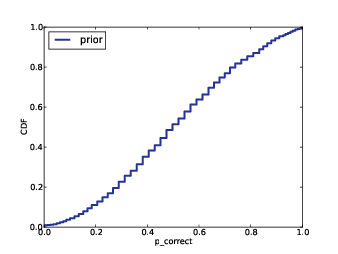
Figure 12.1 shows the prior distribution of p_correct. This distribution is approximately normal, but it is compressed at the extremes. By design, the SAT has the most power to discriminate between test-takers within two standard deviations of the mean, and less power outside that range.

For each test-taker, I define a Suite called Sat that represents the distribution of p_correct. Here’s the definition:

class Sat(thinkbayes.Suite):

    def __init__(self, exam, score):
        thinkbayes.Suite.__init__(self)

        self.exam = exam
        self.score = score

        # start with the prior distribution
        for p_correct, prob in exam.prior.Items():
            self.Set(p_correct, prob)

        # update based on an exam score
        self.Update(score)

__init__ takes an Exam object and a scaled score. It makes a copy of the prior distribution and then updates itself based on the exam score.

As usual, we inherit Update from Suite and provide Likelihood:

    def Likelihood(self, hypo, data):
        p_correct = hypo
        score = data

        raw = self.exam.Reverse(score)
        yes, no = raw, 54 - raw

        like = thinkbayes.EvalBinomialPmf(p_correct, yes, no)
        return like

And as usual, Likelihood computes the likelihood of the data under a given hypothesis. In this case hypo is a hypothetical value of p_correct. And data is a scaled score.

To keep things simple, I interpret the raw score as the number of correct answers, ignoring the penalty for wrong answers. With this simplification, the likelihood is given by the binomial distribution, which computes the probability of yes correct answers and no incorrect.

12.4 Posterior

Figure 12.2: Posterior distributions of p_correct for Alice and Bob.

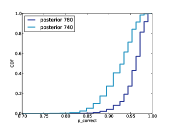
Figure 12.2 shows the posterior distributions of p_correct for Alice and Bob based on their exam scores. We can see that they overlap, so it is possible that p_correct is actually higher for Bob, but it looks unlikely.

Which brings us back to the original question, “How strong is the evidence that Alice is better prepared than Bob?” We can use the posterior distributions of p_correct to answer this question.

To formulate the question in terms of Bayesian hypothesis testing, I define two hypotheses:

A: p_correct is higher for Alice than for Bob.
B: p_correct is higher for Bob than for Alice.

To compute the likelihood of A, we can enumerate all pairs of values from the posterior distributions, and add up the total probability of the cases where p_correct is higher for Alice than for Bob. And we already have a function, thinkbayes.PmfProbGreater that does that.

So we can define a Suite that computes the posterior probabilities of A and B:

class TopLevel(thinkbayes.Suite):

    def Update(self, data):
        a_sat, b_sat = data

        a_like = thinkbayes.PmfProbGreater(a_sat, b_sat)
        b_like = thinkbayes.PmfProbLess(a_sat, b_sat)
        c_like = thinkbayes.PmfProbEqual(a_sat, b_sat)

        a_like += c_like / 2
        b_like += c_like / 2

        self.Mult('A', a_like)
        self.Mult('B', b_like)

        self.Normalize()

Usually when we define a new Suite, we inherit Update and provide Likelihood. In this case I override Update, because it is easier to evaluate the likelihood of both hypotheses at the same time.

The data passed to Update are Sat objects that represent the posterior distributions of p_correct.

a_like is the total probability that p_correct is higher for Alice; b_like is that probability that it is higher for Bob.

c_like is the probability that they are “equal,” but this equality is an artifact of the decision to model p_correct with a set of discrete values. If we chose more values, c_like would be smaller, and in the extreme, if p_correct were continuous, c_like would be zero. So I treat c_like as a kind of round-off error, and split it evenly between a_like and b_like.

Here is the code that creates TopLevel and updates it:

    exam = Exam()
    a_sat = Sat(exam, 780)
    b_sat = Sat(exam, 740)

    top = TopLevel('AB')
    top.Update((a_sat, b_sat))
    top.Print()

The likelihood of A is 0.79 and the likelihood of B is 0.21. The likelihood ratio (or Bayes factor) is 3.8, which means that these test scores are evidence that Alice is better than Bob at answering SAT questions. If we believed, before seeing the test scores, that A and B were equally likely, then after seeing the scores we should believe that the probability of A is 79%, which means there is still an 21% chance that Bob is actually better prepared.

12.5 A better model

Remember that the analysis we have done so far is based on the simplification that all SAT questions are equally difficult. In reality, some are easier than others, which means that the difference between Alice and Bob might be even smaller.

To see why, consider a test where most questions are so easy that Alice and Bob are nearly certain to answer them correctly. In that case, the difference between their scores is determined by a small number of difficult questions, so it is more likely to be due to chance.

But how big is the modeling error? If it is small, we conclude that the first model—based on the simplification that all questions are equally difficult—is good enough. If it’s large, we need a better model.

In the next few sections, I develop a better model and we will discover (spoiler alert!) that the modeling error is small. So if you are satisfied with the simpler mode, you can skip to the next chapter. If you want to see how the more realistic model works, read on...

First, let’s assume that each test-taker has some degree of efficacy, that measures their ability to answer SAT questions.
Second, assume that each question has some level of difficulty.
Finally, assume that the chance that a test-taker answers a question correctly is related to efficacy and difficulty according to this function:
```
def ProbCorrect(efficacy, difficulty, a=1):
    return 1 / (1 + math.exp(-a * (efficacy - difficulty)))
```

This function is a simplified version of the curve used in item response theory, which you can read about at http://en.wikipedia.org/wiki/Item_response_theory. efficacy and difficulty are considered to be on the same scale, and the probability of getting a question right depends only on the difference between them.

When efficacy and difficulty are equal, the probability of getting the question right is 50%. As efficacy increases, this probability approaches 100%. As it decreases (or as difficulty increases), the probability approaches 0%.

Given the distribution of efficacy across test-takers and the distribution of difficulty across questions, we can compute the expected distribution of raw scores. We’ll do that in two steps. First, for a person with given efficacy, we’ll compute the distribution of raw scores.

def PmfCorrect(efficacy, difficulties):
    pmf0 = thinkbayes.Suite([0])

    ps = [ProbCorrect(efficacy, diff) for diff in difficulties]
    pmfs = [BinaryPmf(p) for p in ps]
    dist = sum(pmfs, pmf0)
    return dist

difficulties is a list of difficulties, one for each question. ps is a list of probabilities, and pmfs is a list of two-valued Pmf objects; here’s the function that makes them:

def BinaryPmf(p):
    pmf = thinkbayes.Pmf()
    pmf.Set(1, p)
    pmf.Set(0, 1-p)
    return pmf

dist is the sum of these Pmfs. Remember from Section 5.4 that when we add up Pmf objects, the result is the distribution of the sums. In order to use Python’s sum to add up Pmfs, we have to provide pmf0 which is the identity for Pmfs, so pmf + pmf0 is always pmf.

So if we know a person’s efficacy, we can compute their distribution of raw scores. For a group of people with a different efficacies, the resulting distribution of raw scores is a mixture. Here’s the code that computes the mixture:

class Exam:

    def MakeRawScoreDist(self, efficacies):
        pmfs = thinkbayes.Pmf()
        for efficacy, prob in efficacies.Items():
            scores = PmfCorrect(efficacy, self.difficulties)
            pmfs.Set(scores, prob)

        mix = thinkbayes.MakeMixture(pmfs)
        return mix

efficacies is a Pmf that represents the distribution of efficacy across test-takers. I assume that it is Gaussian with mean 0 and standard deviation 1.5. This choice is mostly arbitrary. The probability of getting a question correct depends on the difference between efficacy and difficulty, so we can choose the units of efficacy and then calibrate the units of difficulty accordingly.

pmfs is a Meta-Pmf that contains one Pmf for each level of efficacy, and maps to the fraction of test-takers at that level. thinkbayes.MakeMixture takes the meta-pmf and compute the distribution of the mixture (see Section 7.4).

12.6 Calibration

If we were given the distribution of difficulty, we could use MakeRawScoreDist to compute the distribution of raw scores. But for us the problem is the other way around: we are given the distribution of raw scores and we want to infer the distribution of difficulty.

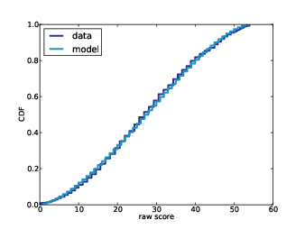
Figure 12.3: Actual distribution of raw scores and a model to fit it.

I assume that the distribution of difficulty is uniform with parameters center and width. MakeDifficulties makes a list of difficulties with these parameters.

def MakeDifficulties(center, width, n):
    low, high = center-width, center+width
    return numpy.linspace(low, high, n)

By trying out a few combinations, I found that the values center=-0.05 and width=1.8 yield a distribution of raw scores similar to the actual data. Figure 12.3 shows the actual data and the results from this model.

So, assuming that the distribution of difficulty is uniform, the range is approximately -1.85 to 1.75, on a scale with a distribution of efficacy that is Gaussian with mean 0 and standard deviation 1.5.

The following table shows the range of ProbCorrect for test-takers at different levels of efficacy:

	Difficulty
Efficacy	-1.85	-0.05	1.75
3.00	0.99	0.95	0.78
1.50	0.97	0.82	0.44
0.00	0.86	0.51	0.15
-1.50	0.59	0.19	0.04
-3.00	0.24	0.05	0.01

Someone with efficacy 3 (two standard deviations above the mean) has a 99% chance of answering the easiest questions on the exam, and a 78% chance of answering the hardest. On the other end of the range, someone two standard deviations below the mean has only a 24% chance of answering the easiest questions.

12.7 Posterior distribution of efficacy

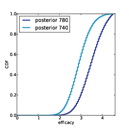
Figure 12.4: Posterior distributions of efficacy for Alice and Bob.

Now that the model is calibrated, we can compute the posterior distribution of efficacy for Alice and Bob. Here is a version of the Sat class that works with the new model:

class Sat2(thinkbayes.Suite):

    def __init__(self, exam, score):
        thinkbayes.Suite.__init__(self)

        self.exam = exam
        self.score = score

        # start with the prior distribution
        efficacies = thinkbayes.MakeGaussianPmf(0, 1.5, 3)
        for efficacy, prob in efficacies.Items():
            self.Set(efficacy, prob)

        # update based on an exam score
        self.Update(score)

The prior distribution of efficacy is Gaussian with mean 0 and standard deviation 1.5 (and the suite of hypotheses spans 3 standard deviations in each direction).

Sat2.Likelihood computes the likelihood of a given test score for a hypothetical level of efficacy.

    def Likelihood(self, hypo, data):
        efficacy = hypo
        score = data
        raw = self.exam.Reverse(score)

        pmf = self.exam.PmfCorrect(efficacy)
        like = pmf.Prob(raw)
        return like

pmf is the distribution of raw scores for a test-taker with the given efficacy; like is the probability of the observed score.

Figure 12.4 shows the posterior distributions of efficacy for Alice and Bob. As expected, the location of Alice’s distribution is farther to the right, but again there is some overlap.

Using TopLevel again, we compare A, the hypothesis that Alice’s efficacy is higher, and B, the hypothesis that Bob’s is higher. The likelihood ratio is 3.4, a bit smaller than what we got from the simple model (3.8). So this model indicates that the data are evidence in favor of A, but a little weaker than the previous estimate.

If our prior belief is that A and B are equally likely, then in light of this evidence we would give A a posterior probability of 77%, leaving a 23% chance that Bob’s efficacy is higher.

12.8 Predictive distribution

The analysis we have done so far generates estimates for Alice and Bob’s efficacy, but since efficacy is not directly observable, it is hard to validate the results.

To give the model predictive power, we can use it to answer another related question: “If Alice and Bob take the math SAT again, what is the chance that Alice will do better again?”

We’ll answer this question in two steps:

We’ll use the posterior distribution of efficacy to generate a predictive distribution of raw score for each test-taker.
We’ll compare the two predictive distributions to compute the probability that Alice gets a higher score again.

We already have most of the code we need. To compute the predictive distributions, we can use MakeRawScoreDist again:

    exam = Exam()
    a_sat = Sat(exam, 780)
    b_sat = Sat(exam, 740)

    a_pred = exam.MakeRawScoreDist(a_sat)
    b_pred = exam.MakeRawScoreDist(b_sat)

Then we can find the likelihood that Alice does better on the second test, Bob does better, or they tie:

    a_like = thinkbayes.PmfProbGreater(a_pred, b_pred)
    b_like = thinkbayes.PmfProbLess(a_pred, b_pred)
    c_like = thinkbayes.PmfProbEqual(a_pred, b_pred)

The probability that Alice does better on the second exam is 63%, which means that Bob has a 37% chance of doing as well or better.

Notice that we have more confidence about Alice’s efficacy than we do about the outcome of the next test. The posterior odds are 3:1 that Alice’s efficacy is higher, but only 2:1 that Alice will do better on the next exam.

12.9 Nuisance parameters

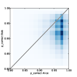
Figure 12.5: Joint posterior distribution of p_correct for Alice and Bob.

In this chapter we started with the question, “How strong is the evidence that Alice is better prepared than Bob?” On the face of it, that sounds like we want to test two hypotheses: either Alice is more prepared or Bob is.

But in order to compute likelihoods for these hypotheses, we have to solve an estimation problem. For each test-taker we have to find the posterior distribution of either p_correct or efficacy.

We don’t really care about these values, but we have to estimate them to solve the problem we care about. Which is why values like this are called “nuisance parameters.”

One way to visualize the analysis we did in this chapter is to plot the space of these parameters. thinkbayes.JointPmf takes two Pmfs, computes their joint distribution, and returns a Pmf of each possible pair of values and its probability.

def JointPmf(pmf1, pmf2):
    pmf = Pmf()
    for v1, p1 in pmf1.Items():
        for v2, p2 in pmf2.Items():
            pmf.Set((v1, v2), p1 * p2)
    return pmf

This function assumes that the two distributions are independent.

Figure 12.5 shows the joint posterior distribution of p_correct for Alice and Bob. The diagonal like indicates the part of the space where p_correct is the same for Alice and Bob. To the right of this line, Alice is more prepared; to the left Bob is more prepared.

In TopLevel.Update, when we computed the likelihoods of A and B, we added up the probability mass each side of this line. For the cells that fall on the line, we added up the total mass and split it between A and B.

The process we used in this chapter—estimating a nuisance variable in order to evaluate the likelihood of competing hypotheses—is a common Bayesian approach to problems like this.

Are you using one of our books in a class?

We'd like to know about it. Please consider filling out this short survey.