Chapter 14  A Hierarchical Model

14.1  The Geiger counter problem

I got the idea for the following problem from Tom Campbell-Ricketts, author of the Maximum Entropy blog at http://maximum-entropy-blog.blogspot.com. And he got the idea from E. T. Jaynes, author of the classic Probability Theory: The Logic of Science:

Suppose that a radioactive source emits particles toward a Geiger counter at an average rate of r particles per second, but the counter only registers a fraction, f, of the particles that hit it. If f is 10% and the counter registers 15 particles in a one second interval, what is the posterior distribution of n, the actual number of particles that hit the counter, and r, the average rate particles are emitted?

To get started on a problem like this, think about the chain of causation that starts with the parameters of the system and ends with the observed data:

1. The source emits particles at an average rate, r.
2. During any given second, the source emits n particles toward the counter.
3. Out of those n particles, some number, k, get counted.

The probability that an atom decays is the same at any point in time, so radioactive decay is well modeled by a Poisson process. Given r, the distribution of n is Poisson distribution with parameter r.

And if we assume that the probability of detection for each particle is independent of the others, the distribution of k is the binomial distribution with parameters n and f.

Given the parameters of the system, we can find the distribution of the data. So we can solve what is called the forward problem.

Now we want to go the other way: given the data, we want the distribution of the parameters. This is called the inverse problem. And if you can solve the forward problem, you can use Bayesian methods to solve the inverse problem.

14.2  Start simple

---

Figure 14.1: Posterior distribution of n for three values of r.

---

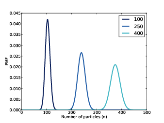
Let’s start with a simple version of the problem where we know the value of r. We are given the value of f, so all we have to do is estimate n.

I define a Suite called Detector that models the behavior of the detector and estimates n.

class Detector(thinkbayes.Suite):

    def __init__(self, r, f, high=500, step=1):
        pmf = thinkbayes.MakePoissonPmf(r, high, step=step)
        thinkbayes.Suite.__init__(self, pmf, name=r)
        self.r = r
        self.f = f

If the average emission rate is r particles per second, the distribution of n is Poisson with parameter r. high and step determine the upper bound for n and the step size between hypothetical values.

Now we need a likelihood function:

# class Detector

    def Likelihood(self, data, hypo):
        k = data
        n = hypo
        p = self.f

        return thinkbayes.EvalBinomialPmf(k, n, p)

data is the number of particles detected, and hypo is the hypothetical number of particles emitted, n.

If there are actually n particles, and the probability of detecting any one of them is f, the probability of detecting k particles is given by the binomial distribution.

That’s it for the Detector. We can try it out for a range of values of r:

    f = 0.1
    k = 15

    for r in [100, 250, 400]:
        suite = Detector(r, f, step=1)
        suite.Update(k)
        print suite.MaximumLikelihood()

Figure 14.1 shows the posterior distribution of n for several given values of r.

14.3  Make it hierarchical

In the previous section, we assume r is known. Now let’s relax that assumption. I define another Suite, called Emitter, that models the behavior of the emitter and estimates r:

class Emitter(thinkbayes.Suite):

    def __init__(self, rs, f=0.1):
        detectors = [Detector(r, f) for r in rs]
        thinkbayes.Suite.__init__(self, detectors)

rs is a sequence of hypothetical value for r. detectors is a sequence of Detector objects, one for each value of r. The values in the Suite are Detectors, so Emitter is a meta-Suite; that is, a Suite that contains other Suites as values.

To update the Emitter, we have to compute the likelihood of the data under each hypothetical value of r. But each value of r is represented by a Detector that contains a range of values for n.

To compute the likelihood of the data for a given Detector, we loop through the values of n and add up the total probability of k. That’s what SuiteLikelihood does:

# class Detector

    def SuiteLikelihood(self, data):
        total = 0
        for hypo, prob in self.Items():
            like = self.Likelihood(data, hypo)
            total += prob * like
        return total

Now we can write the Likelihood function for the Emitter:

# class Emitter

    def Likelihood(self, data, hypo):
        detector = hypo
        like = detector.SuiteLikelihood(data)
        return like

Each hypo is a Detector, so we can invoke SuiteLikelihood to get the likelihood of the data under the hypothesis.

After we update the Emitter, we have to update each of the Detectors, too.

# class Emitter

    def Update(self, data):
        thinkbayes.Suite.Update(self, data)
        
        for detector in self.Values():
            detector.Update()

A model like this, with multiple levels of Suites, is called hierarchical.

14.4  A little optimization

You might recognize SuiteLikelihood; we saw it in Section 11.2. At the time, I pointed out that we didn’t really need it, because the total probability computed by SuiteLikelihood is exactly the normalizing constant computed and returned by Update.

So instead of updating the Emitter and then updating the Detectors, we can do both steps at the same time, using the result from Detector.Update as the likelihood of Emitter.

Here’s the streamlined version of Emitter.Likelihood:

# class Emitter

    def Likelihood(self, data, hypo):
        return hypo.Update(data)

And with this version of Likelihood we can use the default version of Update. So this version has fewer lines of code, and it runs faster because it does not compute the normalizing constant twice.

14.5  Extracting the posteriors

---

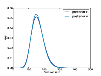
Figure 14.2: Posterior distributions of n and r.

---

After we update the Emitter, we can get the posterior distribution of r by looping through the Detectors and their probabilities:

# class Emitter

    def DistOfR(self):
        items = [(detector.r, prob) for detector, prob in self.Items()]
        return thinkbayes.MakePmfFromItems(items)

items is a list of values of r and their probabilities. The result is the Pmf of r.

To get the posterior distribution of n, we have to compute the mixture of the Detectors. We can use thinkbayes.MakeMixture, which takes a meta-Pmf that maps from each distribution to its probability. And that’s exactly what the Emitter is:

# class Emitter

    def DistOfN(self):
        return thinkbayes.MakeMixture(self)

Figure 14.2 shows the results. Not surprisingly, the most likely value for n is 150. Given f and n, the expected count is k = f n, so given f and k, the expected value of n is k / f, which is 150.

And if 150 particles are emitted in one second, the most likely value of r is 150 particles per second. So the posterior distribution of r is also centered on 150.

The posterior distributions of r and n are similar; the only difference is that we are slightly less certain about n. In general, we can be more certain about the long-range emission rate, r, than about the number of particles emitted in any particular second, n.

You can download the code in this chapter from http://thinkbayes.com/jaynes.py. For more information see Section 0.3.

14.6  Discussion

The Geiger counter problem demonstrates the connection between causation and hierarchical modeling. In the example, the emission rate r has a causal effect on the number of particles, n, which has a causal effect on the particle count, k.

The hierarchical model reflects the structure of the system, with causes at the top and effects at the bottom.

1. At the top level, we start with a range of hypothetical values for r.
2. For each value of r, we have a range of values for n, and the prior distribution of n depends on r.
3. When we update the model, we go bottom-up. We compute a posterior distribution of n for each value of r, then compute the posterior distribution of r.

So causal information flows down the hierarchy, and inference flows up.

14.7  Exercises

Are you using one of our books in a class?

We'd like to know about it. Please consider filling out this short survey.

Think Bayes

Think Python

Think Stats

Think Complexity