This HTML version of is provided for convenience, but it is not the best format for the book. In particular, some of the symbols are not rendered correctly.

You might prefer to read the PDF version, or you can buy a hardcopy here.

Chapter 7  Hypothesis testing

Exploring the data from the NSFG, we saw several “apparent effects,” including a number of differences between first babies and others. So far we have taken these effects at face value; in this chapter, finally, we put them to the test.

The fundamental question we want to address is whether these effects are real. For example, if we see a difference in the mean pregnancy length for first babies and others, we want to know whether that difference is real, or whether it occurred by chance.

That question turns out to be hard to address directly, so we will proceed in two steps. First we will test whether the effect is significant, then we will try to interpret the result as an answer to the original question.

In the context of statistics, “significant” has a technical definition that is different from its use in common language. As defined earlier, an apparent effect is statistically significant if it is unlikely to have occurred by chance.

To make this more precise, we have to answer three questions:

1. What do we mean by “chance”?
2. What do we mean by “unlikely”?
3. What do we mean by “effect”?

All three of these questions are harder than they look. Nevertheless, there is a general structure that people use to test statistical significance:

Null hypothesis:

The null hypothesis is a model of the system based on the assumption that the apparent effect was actually due to chance.

p-value:

The p-value is the probability of the apparent effect under the null hypothesis.

Interpretation:

Based on the p-value, we conclude that the effect is either statistically significant, or not.

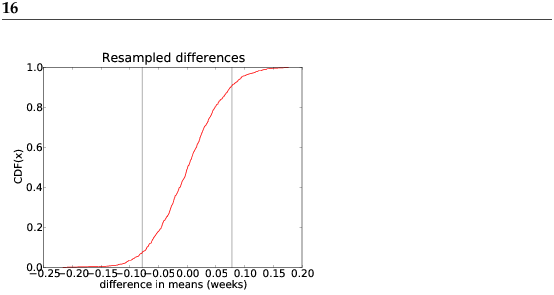
This process is called hypothesis testing. The underlying logic is similar to a proof by contradiction. To prove a mathematical statement, A, you assume temporarily that A is false. If that assumption leads to a contradiction, you conclude that A must actually be true.

Similarly, to test a hypothesis like, “This effect is real,” we assume, temporarily, that is is not. That’s the null hypothesis. Based on that assumption, we compute the probability of the apparent effect. That’s the p-value. If the p-value is low enough, we conclude that the null hypothesis is unlikely to be true.

7.1  Testing a difference in means

One of the easiest hypotheses to test is an apparent difference in mean between two groups. In the NSFG data, we saw that the mean pregnancy length for first babies is slightly longer, and the mean weight at birth is slightly smaller. Now we will see if those effects are significant.

For these examples, the null hypothesis is that the distributions for the two groups are the same, and that the apparent difference is due to chance.

To compute p-values, we find the pooled distribution for all live births (first babies and others), generate random samples that are the same size as the observed samples, and compute the difference in means under the null hypothesis.

If we generate a large number of samples, we can count how often the difference in means (due to chance) is as big or bigger than the difference we actually observed. This fraction is the p-value.

For pregnancy length, we observed n = 4413 first babies and m = 4735 others, and the difference in mean was δ = 0.078 weeks. To approximate the p-value of this effect, I pooled the distributions, generated samples with sizes n and m and computed the difference in mean.

This is another example of resampling, because we are drawing a random sample from a dataset that is, itself, a sample of the general population. I computed differences for 1000 sample pairs; Figure 7.1 shows their distribution.

---

Figure 7.1: CDF of difference in mean for resampled data.

---

The mean difference is near 0, as you would expect with samples from the same distribution. The vertical lines show the cutoffs where x = −δ or x = δ.

Of 1000 sample pairs, there were 166 where the difference in mean (positive or negative) was as big or bigger than δ, so the p-value is approximately 0.166. In other words, we expect to see an effect as big as δ about 17% of the time, even if the actual distribution for the two groups is the same.

So the apparent effect is not very likely, but is it unlikely enough? I’ll address that in the next section.

7.2  Choosing a threshold

In hypothesis testing we have to worry about two kinds of errors.

• A Type I error, also called a false positive, is when we accept a hypothesis that is actually false; that is, we consider an effect significant when it was actually due to chance.
• A Type II error, also called a false negative, is when we reject a hypothesis that is actually true; that is, we attribute an effect to chance when it was actually real.

The most common approach to hypothesis testing is to choose a threshold¹, α, for the p-value and to accept as significant any effect with a p-value less than α. A common choice for α is 5%. By this criterion, the apparent difference in pregnancy length for first babies is not significant, but the difference in weight is.

For this kind of hypothesis testing, we can compute the probability of a false positive explicitly: it turns out to be α.

To see why, think about the definition of false positive—the chance of accepting a hypothesis that is false—and the definition of a p-value—the chance of generating the measured effect if the hypothesis is false.

Putting these together, we can ask: if the hypothesis is false, what is the chance of generating a measured effect that will be considered significant with threshold α? The answer is α.

We can decrease the chance of a false positive by decreasing the threshold. For example, if the threshold is 1%, there is only a 1% chance of a false positive.

But there is a price to pay: decreasing the threshold raises the standard of evidence, which increases the chance of rejecting a valid hypothesis.

In general there is a tradeoff between Type I and Type II errors. The only way to decrease both at the same time is to increase the sample size (or, in some cases, decrease measurement error).

7.3  Defining the effect

When something unusual happens, people often say something like, “Wow! What were the chances of that?” This question makes sense because we have an intuitive sense that some things are more likely than others. But this intuition doesn’t always hold up to scrutiny.

For example, suppose I toss a coin 10 times, and after each toss I write down H for heads and T for tails. If the result was a sequence like THHTHTTTHH, you wouldn’t be too surprised. But if the result was HHHHHHHHHH, you would say something like, “Wow! What were the chances of that?”

But in this example, the probability of the two sequences is the same: one in 1024. And the same is true for any other sequence. So when we ask, “What were the chances of that,” we have to be careful about what we mean by “that.”

For the NSFG data, I defined the effect as “a difference in mean (positive or negative) as big or bigger than δ.” By making this choice, I decided to evaluate the magnitude of the difference, ignoring the sign.

A test like that is called two-sided, because we consider both sides (positive and negative) in the distribution from Figure 7.1. By using a two-sided test we are testing the hypothesis that there is a significant difference between the distributions, without specifying the sign of the difference.

The alternative is to use a one-sided test, which asks whether the mean for first babies is significantly higher than the mean for others. Because the hypothesis is more specific, the p-value is lower—in this case it is roughly half.

7.4  Interpreting the result

At the beginning of this chapter I said that the question we want to address is whether an apparent effect is real. We started by defining the null hypothesis, denoted H₀, which is the hypothesis that the effect is not real. Then we defined the p-value, which is P(E|H₀), where E is an effect as big as or bigger than the apparent effect. Then we computed p-values and compared them to a threshold, α.

That’s a useful step, but it doesn’t answer the original question, which is whether the effect is real. There are several ways to interpret the result of a hypothesis test:

Classical:

In classical hypothesis testing, if a p-value is less than α, you can say that the effect is statistically significant, but you can’t conclude that it’s real. This formulation is careful to avoid leaping to conclusions, but it is deeply unsatisfying.

Practical:

In practice, people are not so formal. In most science journals, researchers report p-values without apology, and readers interpret them as evidence that the apparent effect is real. The lower the p-value, the higher their confidence in this conclusion.

Bayesian:

What we really want to know is P(H_A|E), where H_A is the hypothesis that the effect is real. By Bayes’s theorem

P(HA  |  E) =

P(E  |  HA)   P(HA) P(E)

where P(H_A) is the prior probability of H_A before we saw the effect, P(E|H_A) is the probability of seeing E, assuming that the effect is real, and P(E) is the probability of seeing E under any hypothesis. Since the effect is either real or it’s not,

   P(E) = P(E|H_A) P(H_A) + P(E|H₀) P(H₀)

As an example, I’ll compute P(H_A|E) for pregnancy lengths in the NSFG. We have already computed P(E|H₀) = 0.166, so all we have to do is compute P(E|H_A) and choose a value for the prior.

To compute P(E|H_A), we assume that the effect is real—that is, that the difference in mean duration, δ, is actually what we observed, 0.078. (This way of formulating H_A is a little bit bogus. I will explain and fix the problem in the next section.)

By generating 1000 sample pairs, one from each distribution, I estimated P(E|H_A) = 0.494. With the prior P(H_A) = 0.5, the posterior probability of H_A is 0.748.

So if the prior probability of H_A is 50%, the updated probability, taking into account the evidence from this dataset, is almost 75%. It makes sense that the posterior is higher, since the data provide some support for the hypothesis. But it might seem surprising that the difference is so large, especially since we found that the difference in means was not statistically significant.

In fact, the method I used in this section is not quite right, and it tends to overstate the impact of the evidence. In the next section we will correct this tendency.

7.5  Cross-validation

In the previous example, we used the dataset to formulate the hypothesis H_A, and then we used the same dataset to test it. That’s not a good idea; it is too easy to generate misleading results.

The problem is that even when the null hypothesis is true, there is likely to be some difference, δ, between any two groups, just by chance. If we use the observed value of δ to formulate the hypothesis, P(H_A|E) is likely to be high even when H_A is false.

We can address this problem with cross-validation, which uses one dataset to compute δ and a different dataset to evaluate H_A. The first dataset is called the training set; the second is called the testing set.

In a study like the NSFG, which studies a different cohort in each cycle, we can use one cycle for training and another for testing. Or we can partition the data into subsets (at random), then use one for training and one for testing.

I implemented the second approach, dividing the Cycle 6 data roughly in half. I ran the test several times with different random partitions. The average posterior probability was P(H_A|E) = 0.621. As expected, the impact of the evidence is smaller, partly because of the smaller sample size in the test set, and also because we are no longer using the same data for training and testing.

7.6  Reporting Bayesian probabilities

In the previous section we chose the prior probability P(H_A) = 0.5. If we have a set of hypotheses and no reason to think one is more likely than another, it is common to assign each the same probability.

Some people object to Bayesian probabilities because they depend on prior probabilities, and people might not agree on the right priors. For people who expect scientific results to be objective and universal, this property is deeply unsettling.

One response to this objection is that, in practice, strong evidence tends to swamp the effect of the prior, so people who start with different priors will converge toward the same posterior probability.

Another option is to report just the likelihood ratio, P(E | H_A)  /  P(E|H₀), rather than the posterior probability. That way readers can plug in whatever prior they like and compute their own posteriors (no pun intended). The likelihood ratio is sometimes called a Bayes factor (see http://wikipedia.org/wiki/Bayes_factor).

7.7  Chi-square test

In Section 7.2 we concluded that the apparent difference in mean pregnancy length for first babies and others was not significant. But in Section 2.10, when we computed relative risk, we saw that first babies are more likely to be early, less likely to be on time, and more likely to be late.

So maybe the distributions have the same mean and different variance. We could test the significance of the difference in variance, but variances are less robust than means, and hypothesis tests for variance often behave badly.

An alternative is to test a hypothesis that more directly reflects the effect as it appears; that is, the hypothesis that first babies are more likely to be early, less likely to be on time, and more likely to be late.

We proceed in five easy steps:

1. We define a set of categories, called cells, that each baby might fall into. In this example, there are six cells because there are two groups (first babies and others) and three bins (early, on time or late).

   I’ll use the definitions from Section 2.10: a baby is early if it is born during Week 37 or earlier, on time if it is born during Week 38, 39 or 40, and late if it is born during Week 41 or later.

2. We compute the number of babies we expect in each cell. Under the null hypothesis, we assume that the distributions are the same for the two groups, so we can compute the pooled probabilities: P(early), P(ontime) and P(late).

   For first babies, we have n = 4413 samples, so under the null hypothesis we expect n P(early) first babies to be early, n P(ontime) to be on time, etc. Likewise, we have m = 4735 other babies, so we expect m P(early) other babies to be early, etc.

3. For each cell we compute the deviation; that is, the difference between the observed value, O_i, and the expected value, E_i.
4. We compute some measure of the total deviation; this quantity is called the test statistic. The most common choice is the chi-square statistic:

   χ2 =

   ∑ i

   (Oi − Ei)2 Ei

5. We can use a Monte Carlo simulation to compute the p-value, which is the probability of seeing a chi-square statistic as high as the observed value under the null hypothesis.

When the chi-square statistic is used, this process is called a chi-square test. One feature of the chi-square test is that the distribution of the test statistic can be computed analytically.

Using the data from the NSFG I computed χ² = 91.64, which would occur by chance about one time in 10,000. I conclude that this result is statistically significant, with one caution: again we used the same dataset for exploration and testing. It would be a good idea to confirm this result with another dataset.

You can download the code I used in this section from http://thinkstats.com/chi.py.

7.8  Efficient resampling

Anyone reading this book who has prior training in statistics probably laughed when they saw Figure 7.1, because I used a lot of computer power to simulate something I could have figured out analytically.

Obviously mathematical analysis is not the focus of this book. I am willing to use computers to do things the “dumb” way, because I think it is easier for beginners to understand simulations, and easier to demonstrate that they are correct. So as long as the simulations don’t take too long to run, I don’t feel guilty for skipping the analysis.

However, there are times when a little analysis can save a lot of computing, and Figure 7.1 is one of those times.

Remember that we were testing the observed difference in the mean between pregnancy lengths for n = 4413 first babies and m = 4735 others. We formed the pooled distribution for all babies, drew samples with sizes n and m, and computed the difference in sample means.

Instead, we could directly compute the distribution of the difference in sample means. To get started, let’s think about what a sample mean is: we draw n samples from a distribution, add them up, and divide by n. If the distribution has mean µ and variance σ², then by the Central Limit Theorem, we know that the sum of the samples is N(nµ, nσ²).

To figure out the distribution of the sample means, we have to invoke one of the properties of the normal distribution: if X is N(µ, σ²),

   aX + b ∼ N(aµ + b, a² σ²)

When we divide by n, a = 1/nand b = 0, so

X/n ∼ N(µ/n, σ²/ n²)

So the distribution of the sample mean is N(µ, σ²/n).

To get the distribution of the difference between two sample means, we invoke another property of the normal distribution: if X₁ is N(µ₁, σ₁²) and X₂ is N(µ₂, σ₂²),

So as a special case:

Putting it all together, we conclude that the sample in Figure 7.1 is drawn from N(0, fσ²), where f = 1/n + 1/m. Plugging in n = 4413 and m = 4735, we expect the difference of sample means to be N(0, 0.0032).

We can use erf.NormalCdf to compute the p-value of the observed difference in the means:

delta = 0.078
sigma = math.sqrt(0.0032)
left = erf.NormalCdf(-delta, 0.0, sigma)
right = 1 - erf.NormalCdf(delta, 0.0, sigma)

The sum of the left and right tails is the p-value, 0.168, which is pretty close to what we estimated by resampling, 0.166. You can download the code I used in this section from http://thinkstats.com/hypothesis_analytic.py

7.9  Power

When the result of a hypothesis test is negative (that is, the effect is not statistically significant), can we conclude that the effect is not real? That depends on the power of the test.

Statistical power is the probability that the test will be positive if the null hypothesis is false. In general, the power of a test depends on the sample size, the magnitude of the effect, and the threshold α.

One way to report the power of a test, along with a negative result, is to say something like, “If the apparent effect were as large as x, this test would reject the null hypothesis with probability p.”

7.10  Glossary

significant:

An effect is statistically significant if it is unlikely to occur by chance.

null hypothesis:

A model of a system based on the assumption that an apparent effect is due to chance.

p-value:

The probability that an effect could occur by chance.

hypothesis testing:

The process of determining whether an apparent effect is statistically significant.

false positive:

The conclusion that an effect is real when it is not.

false negative:

The conclusion that an effect is due to chance when it is not.

two-sided test:

A test that asks, “What is the chance of an effect as big as the observed effect, positive or negative?”

one-sided test:

A test that asks, “What is the chance of an effect as big as the observed effect, and with the same sign?”

cross-validation:

A process of hypothesis testing that uses one dataset for exploratory data analysis and another dataset for testing.

training set:

A dataset used to formulate a hypothesis for testing.

testing set:

A dataset used for testing.

test statistic:

A statistic used to measure the deviation of an apparent effect from what is expected by chance.

chi-square test:

A test that uses the chi-square statistic as the test statistic.

likelihood ratio:

The ratio of P(E|A) to P(E|B) for two hypotheses A and B, which is a way to report results from a Bayesian analysis without depending on priors.

cell:

In a chi-square test, the categories the observations are divided into.

power:

The probability that a test will reject the null hypothesis if it is false.

1

Also known as a “Significance criterion.”

Like this book?

Are you using one of our books in a class?

Think Bayes

Think Python

Think Stats

Think Complexity